
A graph can suggest that a series depends on its past, but it gives no number to compare across series or to test. At each lag \(k\) we need the correlation between the process now and \(k\) periods earlier, estimated from the one history we observe. That correlation is the autocorrelation; the correlogram plots its estimates lag by lag.
In this lesson
- From a graph to a number
- The autocorrelation of a process
- The sample autocorrelation, r(k)
- r(1) by hand: eight quarters
- How much data does r(k) need?
- The band: testing one lag at a time
- Reading a real correlogram: UK GDP growth
- Several lags at once: the Q-test
- Four real correlograms
- Common mistakes
- Check your understanding: five marked questions
- Three questions about autocorrelation
- Where next
1. From a graph to a number
The first step in putting a number on how a series depends on its own past is to plot each value against the value before it. Figure 1 does this for UK GDP growth, the percentage change in real GDP from one quarter to the next (ONS series ABMI, seasonally adjusted, as published in September 2026), over the 144 quarters from 1984 Q1 to 2019 Q4. The 144 quarters give 143 pairs, because the quarter before 1984 Q1 lies outside the sample.
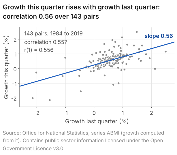
The points rise from left to right: in 98 of the 143 pairs, growth was on the same side of its mean, 0.56% a quarter, as in the quarter before (lesson 22). Their correlation, computed as in lesson 3, is 0.557: one number for what the cloud of points suggests. The line is the least-squares line of lesson 9, the idea behind the AR(1) model that lesson 25 estimates; its slope, 0.56, is close to the correlation only because growth is about as spread out in one column as in the other.
The quarters from 2020 on are left out. Two of them, a fall of 19.9% in 2020 Q2 and a rise of 16.9% in 2020 Q3, would dominate every statistic; with the quarters to 2026 Q2 included, the correlation between successive quarters goes from 0.56 to -0.27 (lesson 22). Every number on this page describes these 144 quarters, not UK GDP growth in general.
The same plot can be drawn at any lag, growth now against growth two, three or more quarters earlier, and each lag gives one correlation. Lesson 22 gave the reason we need these numbers: eye-balling the graph of a series does not tell us the form of the process, nor does it give a way to test between models.
What students say
“Nicky is an excellent econometrics tutor. He explains complex concepts clearly and makes them much easier to understand.”
“I was completely lost in my economics class, and then I started working Nicky and he totally saved me. He was excellent at explaining the material and extremely accommodating to meet with me many times despite us being in different time zones! Highly recommend working with Nicky!”
“Nicky is a very good and thorough teacher. He has excellent knowledge of econometrics and takes the time to work through your questions. Highly recommended!”
“Really great tutor! Encouraging, knowledgeable, friendly”
“Very good lesson, Nicky is very helpful.”
“Very helpful and clear.”
“I gather it was very useful, thank you!”
“Fantastic!”
2. The autocorrelation of a process
The correlation in Figure 1 comes from one history. What it estimates is a feature of the process, the rule that produced this history and could have produced others (lesson 21). We write \(Y_t\) for the process at date \(t\), a random variable, and \(y_1, \dots, y_T\) for the \(T\) numbers we observe, here \(T = 144\).
We are after how strongly the process at date \(t\) moves with itself \(k\) periods earlier; \(k\) is the lag. The autocovariance at lag \(k\) is the covariance of \(Y_t\) and \(Y_{t-k}\) (lesson 3), the average over all possible histories of the product of their deviations from the mean, and the autocorrelation is their correlation. Both assume that the process is stationary: its mean and variance are the same at every date, and the covariance between two dates depends only on how far apart they are (lesson 24). Hence the two standard deviations in that correlation are equal, the autocorrelation is the autocovariance divided by the variance of the process, and it is one number at each lag, the same at every date.
Definition: autocovariance and autocorrelation
For a stationary process \(Y_t\), the autocovariance at lag \(k\), for \(k = 0, 1, 2, \dots\), is
$$ \gamma(k) = \operatorname{Cov}(Y_t, Y_{t-k}) $$and the autocorrelation at lag \(k\) is
$$ \rho(k) = \frac{\gamma(k)}{\gamma(0)} , $$where \(\gamma(0) = \operatorname{Var}(Y_t)\) is the variance of the process. Read as a function of the lag, \(\rho(1), \rho(2), \dots\) is the autocorrelation function (ACF).
Remarks. Intuitively, if \(Y_t\) is GDP growth, \(\rho(1)\) is the correlation between growth this quarter and growth last quarter, taken across all the histories the process could produce, not across the quarters of the one history we have. At lag 0 the process is compared with itself, so \(\rho(0) = 1\). The autocorrelation of the process and the sample autocorrelation of the data (section 3) are not the same thing: the first is a fixed feature of the process, the second an estimate that another history would change.
In words: autocorrelation at lag k = covariance between the process now and k periods earlier, divided by the variance of the process.
Dividing by \(\gamma(0)\) removes the units: a covariance is in the units of the series squared, per cent squared for growth, while \(\rho(k)\), a correlation, has none and lies between -1 and 1 (lesson 3). A white-noise process has \(\rho(k) = 0\) at every lag \(k \ge 1\). A stationary AR(1) with coefficient \(\phi\), the model of lesson 25, has \(\rho(k) = \phi^k\): with \(\phi = 0.5\) these are 0.5, 0.25 and 0.125 at lags 1, 2 and 3. The module note on stationarity, white noise and the ACF sets out the definitions with more algebra.
3. The sample autocorrelation, r(k)
From one history, \(y_1, \dots, y_T\), we estimate \(\rho(k)\). Stationarity again makes this possible: the process has one mean, \(\mu\), and every pair of dates \(k\) apart shares the covariance \(\gamma(k)\). So the \(T - k\) pairs \((y_t, y_{t-k})\) in the sample all carry information on it, and, provided the dependence between distant dates dies away (lesson 24), an average over dates can stand in for the average over histories. The sample autocorrelation at lag \(k\) is
$$ r(k) = \frac{\sum_{t=k+1}^{T}(y_t-\bar y)(y_{t-k}-\bar y)}{\sum_{t=1}^{T}(y_t-\bar y)^2} , $$where \(\bar y = \frac{1}{T}\sum_{t=1}^{T} y_t\) is the mean of all \(T\) observations.
In words: sample autocorrelation at lag k = sum of the products of deviations from the mean, over the pairs k periods apart, divided by the sum of the squared deviations of all T observations.
- One mean, from all \(T\) values. The process has the same mean at every date, so every observation informs its estimate: for the 144 quarters, \(\bar y = 0.561\)% a quarter.
- The numerator starts at \(t = k + 1\), the first date for which the pair \((y_t, y_{t-k})\) is available in the sample. It adds \(T - k\) products: 143 at lag 1 for GDP growth.
- The denominator sums over all \(T\). It estimates the variance of the process, the same at every date, so every observation informs it; divided by \(T\), the numerator and the denominator estimate \(\gamma(k)\) and \(\gamma(0)\), as in \(\rho(k) = \gamma(k)/\gamma(0)\). One denominator for every lag also keeps every \(r(k)\) between -1 and 1.
- No units. Both sums are in the units of the series squared, so the ratio has none.
So \(r(k)\) is not quite the ordinary correlation of the \(T - k\) pairs (lesson 3), which would use a separate mean and a separate sum of squares for each column: for GDP growth at lag 1, the 143 pairs of Figure 1 give 0.557, against \(r(1) = 0.556\). R's acf and statsmodels' acf compute \(r(k)\), and every autocorrelation on this page is computed the same way.
Computed from one history, \(r(k)\) is an estimate: another history of the same length would give another value, and sections 5 and 6 ask how far from \(\rho(k)\) it can lie. We write \(r(k)\); slides and software write \(\hat\rho(k)\) or "AC", and books use other letters again: the choice is cosmetic. The module note on estimation and testing works through \(r(k)\) with more algebra.
4. r(1) by hand: eight quarters
Working the formula through once shows what each part does. Take the eight quarters from 2018 Q1 to 2019 Q4, with growth rounded to one decimal place, the figures the ONS publishes as series IHYQ. Every entry of the table is then exact as printed.
| \(t\) | Quarter | Growth \(y_t\) (%) | Deviation \(d_t = y_t - 0.275\) | \(d_t \times d_{t-1}\) | \(d_t^2\) |
|---|---|---|---|---|---|
| 1 | 2018 Q1 | 0.1 | -0.175 | none | 0.030625 |
| 2 | 2018 Q2 | 0.2 | -0.075 | 0.013125 | 0.005625 |
| 3 | 2018 Q3 | 0.3 | 0.025 | -0.001875 | 0.000625 |
| 4 | 2018 Q4 | 0.1 | -0.175 | -0.004375 | 0.030625 |
| 5 | 2019 Q1 | 0.5 | 0.225 | -0.039375 | 0.050625 |
| 6 | 2019 Q2 | 0.2 | -0.075 | -0.016875 | 0.005625 |
| 7 | 2019 Q3 | 0.6 | 0.325 | -0.024375 | 0.105625 |
| 8 | 2019 Q4 | 0.2 | -0.075 | -0.024375 | 0.005625 |
| Sum | 2.2 | 0 | -0.098125 | 0.235 |
- Mean. The eight values add to 2.2, so \(\bar y = 2.2/8 = 0.275\)% a quarter.
- Deviations. Subtract 0.275 from each value. They add to zero, as deviations from a mean do.
- Products of neighbours. Multiply each deviation by the one before it, from \(t = 2\): the first quarter has no partner. The seven products add to -0.098125.
- Squares. The eight squared deviations add to 0.235.
- Divide. \(r(1) = -0.098125/0.235 = -0.418\).
These eight quarters give a negative \(r(1)\). From 2018 Q3 on, each quarter lies on the other side of the mean from the quarter before, so six of the seven products are negative; the four from 2019 alone add to -0.105. The 144 quarters that contain these eight give +0.556. Read the table as practice in the arithmetic, not as evidence about growth: eight values are too few to settle even the sign of \(\rho(1)\), as sections 5 and 6 show. Rounding also moves the result: with growth unrounded, the same eight quarters give \(r(1) = -0.368\).
5. How much data does r(k) need?
How close \(r(k)\) comes to \(\rho(k)\) depends on the number of observations that go into it. At the extreme, the last three quarters of the table, 0.2, 0.6 and 0.2, give \(r(1) = -2/3 = -0.667\), and algebra settles the range of that number before any data arrive. With three observations the deviations add to zero, so \(d_1 + d_3 = -d_2\), the numerator \(d_2 d_1 + d_3 d_2\) equals \(-d_2^2\), and
$$ r(1) = \frac{-d_2^2}{d_1^2 + d_2^2 + d_3^2} . $$This is never positive, whatever process produced the three numbers, and never below -2/3, its value when \(d_1 = d_3\), as here. Even the steadily rising 1, 2, 3 gives \(r(1) = 0\). With three data points it is difficult to distinguish between different processes.
The lag matters too, since only \(T - k\) pairs enter \(r(k)\). Ten years of annual data leave a single pair at lag 9, the first and the tenth observations, and a correlation from one pair says next to nothing about \(\rho(9)\).
To see how far \(r(k)\) strays from \(\rho(k)\) we need a process whose autocorrelations we know, and in a simulation we set the process ourselves. We draw 10,000 histories of each length \(T = 30\), 100 and 1,000 from the stationary AR(1) with \(\phi = 0.5\) of section 2, for which \(\rho(k) = 0.5^k\), and compute \(r(1)\) to \(r(5)\) in each. Figure 2 shows 100 of them at each length.
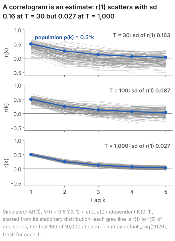
default_rng(2026), fresh for each \(T\), standard_normal((10000, T)).The table gives, for each length, the centre and the spread of the 10,000 values of \(r(1)\).
| Length of each history, \(T\) | 30 | 100 | 1,000 |
|---|---|---|---|
| Mean of \(r(1)\) (\(\rho(1) = 0.5\)) | 0.400 | 0.469 | 0.497 |
| Standard deviation of \(r(1)\) | 0.163 | 0.087 | 0.027 |
| Middle 90% of \(r(1)\) | 0.11 to 0.65 | 0.32 to 0.61 | 0.45 to 0.54 |
At \(T = 30\) one history can show anything from weak dependence to strong: the middle 90% of \(r(1)\) runs from 0.11 to 0.65. The spread falls roughly in proportion to \(1/\sqrt{T}\), as the standard error of a mean does (lesson 5): 1,000 observations are 33.3 times 30, and \(0.163/0.027 = 6.0\), close to \(\sqrt{33.3} = 5.8\).
The centre moves too. At \(T = 30\) the numerator of \(r(1)\) adds 29 products against 30 squares in the denominator, and every deviation is measured from \(\bar y\), which is estimated from the same 30 values; both pull \(r(1)\) towards zero. In this run its mean is 0.400 at \(T = 30\), against \(\rho(1) = 0.5\), rising to 0.469 at \(T = 100\) and 0.497 at \(T = 1{,}000\). So for a positively autocorrelated process, \(r(k)\) is centred below \(\rho(k)\) in small samples.
6. The band: testing one lag at a time
The correlograms on this page draw two dashed lines across the bars, at plus and minus \(1.96/\sqrt{T}\). When the observations are independent and \(T\) is large, \(r(k)\) falls between them by chance in about 95% of samples, so they give a test, lag by lag, of whether \(\rho(k)\) is zero.
- Assumption. The observations are independent, with a constant variance. This is stronger than zero autocorrelation, and the band needs it.
- Result. Each product \((y_t - \bar y)(y_{t-k} - \bar y)\) then has a mean close to zero, and \(r(k)\) is close to an average of \(T - k\) of them, divided by the variance. The variance of such an average falls in proportion to \(1/T\), as a sample mean's does (lesson 4), and a version of the central limit theorem makes it approximately normal. Hence, in a large sample, \(r(k)\) at any one lag \(k \ge 1\) is approximately normal with mean 0 and variance \(1/T\).
- Normal probabilities. A normal distribution has 95% of its probability within 1.96 standard deviations of its centre (lesson 6). Hence \(r(k)\) lies within \(\pm 1.96/\sqrt{T}\) of zero in about 95% of samples.
- Consequence: a test. For \(H_0\): \(\rho(k) = 0\) against \(H_1\): \(\rho(k) \ne 0\) (lesson 7), reject at the 5% level when \(|r(k)| > 1.96/\sqrt{T}\), that is, when \(|\sqrt{T}\, r(k)| > 1.96\). A bar outside the band is evidence against zero autocorrelation at that lag at the 5% level. A bar inside it is no evidence against \(\rho(k) = 0\), which is not the same as evidence that \(\rho(k)\) is zero.
Show where the variance 1/T comes from
Write \(Z_t = Y_t - \mu\) and \(\sigma^2\) for the variance of the process, and take the observations to be independent.
- Simplify. In a large sample \(\bar y\) is close to \(\mu\), and the denominator of \(r(k)\) divided by \(T\) is close to \(\sigma^2\), so $$ r(k) \approx \frac{1}{T\sigma^2}\sum_{t=k+1}^{T} Z_t Z_{t-k} . $$
- One product. By independence, \(E[Z_t Z_{t-k}] = E[Z_t]\,E[Z_{t-k}] = 0\) and \(E[Z_t^2 Z_{t-k}^2] = E[Z_t^2]\,E[Z_{t-k}^2] = \sigma^4\): mean 0, variance \(\sigma^4\).
- Two products. For two dates \(t \ne s\), the latest of \(t\), \(t - k\), \(s\), \(s - k\) appears once in \(Z_t Z_{t-k} Z_s Z_{s-k}\), and its \(Z\) has mean zero and is independent of the rest. So the expectation is zero, and the two products are uncorrelated.
- The sum. The variance of a sum of uncorrelated terms is the sum of their variances (lesson 3), here \((T - k)\sigma^4\). Hence $$ \begin{aligned} \operatorname{Var}\big(r(k)\big) &\approx \frac{(T-k)\,\sigma^4}{T^2\sigma^4} \\ &= \frac{T-k}{T^2} , \end{aligned} $$ a little below \(1/T\): for \(T = 144\) and \(k = 1\), \(143/144^2 = 0.00690\) against \(1/144 = 0.00694\).
Steps 2 and 3 are where independence is used; zero autocorrelation alone would not do. If large values cluster in time, as the size of monthly stock returns does (lesson 22), \(E[Z_t^2 Z_{t-k}^2]\) exceeds \(\sigma^4\) and the band is too narrow.
For the 144 quarters of GDP growth the band is \(\pm 1.96/\sqrt{144} = \pm 1.96/12 = \pm 0.163\), and \(r(1) = 0.556\) lies far outside it: \(\sqrt{144} \times 0.556 = 6.67\), well beyond 1.96. For the eight quarters of section 4 the band is \(\pm 1.96/\sqrt{8} = \pm 0.693\): their \(r(1) = -0.418\) lies inside it, which is no evidence against \(\rho(1) = 0\) and no evidence for it. For three observations the band, \(\pm 1.96/\sqrt{3} = \pm 1.13\), is wider than any correlation can be. Since \(r(k)\) has no units, the band depends only on \(T\), not on the units or the spread of the series.
The 95% holds lag by lag. Since the variance of \(r(k)\) is a little below \(1/T\) and falls with the lag (step 4 of the derivation), a little under one bar in twenty falls outside the band by chance when the observations are independent: for independent normal data with \(T = 144\), 4.8% at lag 1, falling to 4.0% at lag 12. A correlogram shows twelve bars or more, though, and in 10,000 simulated series of 144 independent normal values at least one of twelve bars lay outside the band in 40.3% of them. A single bar narrowly outside the band, among twelve, is weak evidence on its own; section 8 tests the lags together.
Some software draws \(\pm 2/\sqrt{T}\) instead, or a band that widens with the lag and rests on a different null hypothesis; the correlogram explainer compares them. Every correlogram on this page uses \(\pm 1.96/\sqrt{T}\).
7. Reading a real correlogram: UK GDP growth
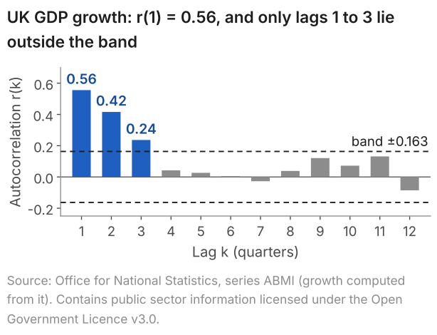
A correlogram sets the sample autocorrelations side by side as bars, one for each lag, with the band drawn across them. First the numbers: the first eight sample autocorrelations of GDP growth over the 144 quarters, against the band of \(\pm 0.163\).
| Lag \(k\) (quarters) | \(r(k)\) | Outside \(\pm 0.163\)? |
|---|---|---|
| 1 | 0.556 | Yes |
| 2 | 0.416 | Yes |
| 3 | 0.237 | Yes |
| 4 | 0.042 | No |
| 5 | 0.027 | No |
| 6 | 0.005 | No |
| 7 | -0.027 | No |
| 8 | 0.039 | No |
Figure 3 draws them, with four more lags.
The code below reads uk-gdp-growth.csv (real GDP in £ million and growth in per cent, quarterly from 1955 Q1); save it in your working folder first. It recomputes growth at full precision from the GDP column, keeps 1984 Q1 to 2019 Q4, and prints \(r(0) = 1\) (the series compared with itself) to \(r(8)\), then the Q-test of section 8.
R: the code
# UK GDP growth (% per quarter), 1984 Q1 to 2019 Q4: autocorrelations and the Ljung-Box Q
gdp <- read.csv("uk-gdp-growth.csv")
# full-precision growth from gdp (the file's growth column has 4 decimals)
gdp$growth <- c(NA, 100 * (gdp$gdp[-1] / head(gdp$gdp, -1) - 1))
g <- gdp$growth[gdp$quarter >= "1984Q1" & gdp$quarter <= "2019Q4"]
length(g)
acf(g, lag.max = 8, plot = FALSE)
Box.test(g, lag = 8, type = "Ljung-Box")
R: what it prints
> # UK GDP growth (% per quarter), 1984 Q1 to 2019 Q4: autocorrelations and the Ljung-Box Q
> gdp <- read.csv("uk-gdp-growth.csv")
> # full-precision growth from gdp (the file's growth column has 4 decimals)
> gdp$growth <- c(NA, 100 * (gdp$gdp[-1] / head(gdp$gdp, -1) - 1))
> g <- gdp$growth[gdp$quarter >= "1984Q1" & gdp$quarter <= "2019Q4"]
> length(g)
[1] 144
> acf(g, lag.max = 8, plot = FALSE)

Autocorrelations of series ‘g’, by lag

     0      1      2      3      4      5      6      7      8
 1.000  0.556  0.416  0.237  0.042  0.027  0.005 -0.027  0.039
> Box.test(g, lag = 8, type = "Ljung-Box")

	Box-Ljung test

data:  g
X-squared = 80.075, df = 8, p-value = 4.718e-14
Python: the code
import pandas as pd
from statsmodels.stats.diagnostic import acorr_ljungbox
from statsmodels.tsa.stattools import acf

# UK GDP growth (% per quarter), 1984 Q1 to 2019 Q4: autocorrelations and the Ljung-Box Q
gdp = pd.read_csv("uk-gdp-growth.csv")
# full-precision growth from gdp (the file's growth column has 4 decimals)
gdp["growth"] = 100 * gdp["gdp"].pct_change()
g = gdp.loc[gdp["quarter"].between("1984Q1", "2019Q4"), "growth"]
print("T =", len(g))
print(acf(g, nlags=8).round(3))  # lags 0 to 8
print(acorr_ljungbox(g, lags=[8]))
Python: what it prints
T = 144
[ 1.     0.556  0.416  0.237  0.042  0.027  0.005 -0.027  0.039]
     lb_stat     lb_pvalue
8  80.075065  4.721701e-14
Lags 1 to 3 lie outside the band, and all three are positive: at each of them there is evidence, at the 5% level, against zero autocorrelation. In these 144 quarters, growth above the mean has gone with growth above the mean one, two and three quarters later. The three decline, 0.556, 0.416 and 0.237, and from lag 4 on every bar lies inside the band, the largest being 0.131 at lag 11.
A stationary AR(1) with a positive coefficient has \(\rho(k) = \phi^k\), which falls by the same factor at each lag (section 2): positive autocorrelations that decline with the lag. That makes an AR(1) one candidate model for these data. An AR(1) with \(\phi = r(1) = 0.556\) would have \(\rho(2) = 0.556^2 = 0.309\) and \(\rho(3) = 0.556^3 = 0.172\); the sample gives 0.416 and 0.237, a slower decline. Each \(r(k)\) is an estimate with its own sampling error (section 5), so the gap does not rule out an AR(1), but it leaves room for models whose autocorrelations fall more slowly, such as an AR(2) or an ARMA(1,1). The correlogram does not test between them: lesson 25 fits the AR(1), the explainer on AR, MA and ARMA models sets out the others, and the correlogram explainer shows how the residuals of a fitted model are checked.
8. Several lags at once: the Q-test
The band tests one lag at a time. The Ljung-Box statistic tests the first \(m\) lags together, \(H_0\): \(\rho(1) = \dots = \rho(m) = 0\) against \(H_1\): at least one of them is not zero, by combining the first \(m\) sample autocorrelations into one number:
$$ Q(m) = T(T+2)\sum_{k=1}^{m}\frac{r(k)^2}{T-k} . $$In words: Q = T(T + 2) times the sum, over lags 1 to m, of each squared sample autocorrelation divided by T - k.
Squaring makes autocorrelations of either sign count against \(H_0\), so \(Q\) is large when any of them is far from zero; the weights \((T + 2)/(T - k)\) are a little above 1, from \(146/143 = 1.02\) to \(146/136 = 1.07\) for \(T = 144\) and \(m = 8\). When the observations are independent, \(Q(m)\) has approximately a chi-square distribution with \(m\) degrees of freedom in a large sample. For GDP growth, \(Q(8) = 80.075\), computed from the unrounded autocorrelations, far above 15.51, the 5% critical value: the point that a chi-square variable with 8 degrees of freedom exceeds with probability 0.05. The p-value, the probability of a \(Q\) at least this large if \(H_0\) is true, is below 0.0005, so we reject \(H_0\) at the 5% level: the data are evidence that at least one of \(\rho(1)\) to \(\rho(8)\) is not zero, not that all eight are; the bars at lags 4 to 8 lie inside the band. The correlogram explainer gives the test in full.
9. Four real correlograms
Each feature that lesson 22 looks for in a graph leaves its own shape in the correlogram. Figure 4 sets four real series side by side, each with its own band, since their lengths differ.
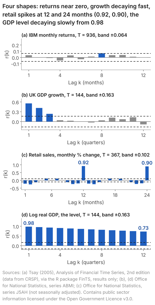
(a) IBM returns: little sign of dependence. Only lag 8 lies outside the band, narrowly, which among twelve bars is weak evidence (section 6); the Q-test of all twelve, \(Q(12) = 12.42\) with a p-value of 0.413, does not reject. Large moves cluster, though (lesson 22), so the size of the returns shows dependence on its past; lesson 24 shows the correlogram of their squared deviations.
(b) GDP growth: decay over three lags, the persistence of lesson 22.
(c) Retail sales: spikes at 12 and 24 months. The change in a month moves with the change in the same month one and two years earlier: the yearly pattern of lesson 22, which a series that is not seasonally adjusted keeps.
(d) The level of log GDP: a slow decline from near 1. Early in the sample the values lie below their mean and late in the sample above it, so values a few quarters apart sit on the same side of the mean, and their products of deviations are positive. That is the mark of a trending level, and it says little about how growth depends on its past. Lesson 24 shows why the level is differenced first. Panel (b) is close to the correlogram of that difference: 100 times the change in log GDP is close to, though not equal to, percentage growth.
10. Common mistakes
- Calling bars "significant" without the test. When I marked an exam question that showed a correlogram, a common mistake was to state that correlations were "significant" without carrying out the test, at each lag or with \(Q\), that shows which are non-zero. Name the test and its level ("\(r(1) = 0.556\) lies outside \(\pm 0.163\): evidence at the 5% level against \(\rho(1) = 0\)"), then describe the pattern, here positive autocorrelations that decline with the lag.
- Reading \(r(k)\) as \(\rho(k)\). The bars are estimates from one history: in the simulation of section 5, \(r(1)\) for a process with \(\rho(1) = 0.5\) had a standard deviation of 0.163 at \(T = 30\).
- "Inside the band, so the autocorrelation is zero." Inside is no evidence against zero, at that lag and the 5% level. In the simulation of section 5, where \(\rho(1) = 0.5\), \(r(1)\) still fell inside the band \(\pm 1.96/\sqrt{30} = \pm 0.358\) in 36.7% of the histories of length 30.
- One bar outside, among twelve, taken as proof of dependence. In 40.3% of simulated independent series of 144, at least one of twelve bars fell outside the band.
- "Positive and declining, so the process is an AR(1)." An AR(1) is one candidate. Compare \(r(2)\) with \(r(1)^2\): for GDP growth, 0.416 against 0.309.
- "The p-value of \(Q\) is the probability that all the autocorrelations are zero." It is the probability of a \(Q\) at least as large as the one observed if they were all zero.
11. Check your understanding
Five questions, marked on the page; every option has an explanation, including the wrong ones. (Without JavaScript the explanations are shown beneath each question.)
1. Five quarters of growth in a made-up economy are 0.8, 0.6, 0.2, 0.4 and 0.5 per cent. What is their sample autocorrelation at lag 1, r(1)?
Correct. The mean is 2.5/5 = 0.5, so the deviations are 0.3, 0.1, -0.3, -0.1 and 0. The four products of neighbours, 0.03, -0.03, 0.03 and 0, add to 0.03; the five squares add to 0.2. So r(1) = 0.03/0.2 = 0.15.
0.23 is the ordinary correlation of the four pairs, with a separate mean for each column (0.5 and 0.425) and separate sums of squares. r(1) uses one mean, 0.5, and the squares of all five deviations: 0.03/0.2 = 0.15.
0.03/0.11 = 0.27 sums the squares over the last four quarters only. The denominator of r(1) estimates the variance from all five deviations, whose squares add to 0.2, so r(1) = 0.03/0.2 = 0.15.
0.88/1.45 = 0.61 multiplies and squares the growth figures themselves. r(1) works with deviations from the mean, 0.5: the products add to 0.03 and the squares to 0.2, which gives 0.15.
2. A monthly series has T = 400 observations, with a mean of 0.6% and a standard deviation of 2.0%. Where should the band of its correlogram be drawn, for a test at the 5% level at each lag?
1.96/400 = 0.0049 divides by T. When the observations are independent, the standard deviation of r(k) is about 1/√T = 1/20 = 0.05, so the band is ±1.96 × 0.05 = ±0.098.
±1/√400 = ±0.05 is one standard deviation of r(k) either side of zero, which holds about 68% of samples, not 95%. The 5% test uses 1.96 standard deviations: ±1.96/20 = ±0.098.
1.645/20 = 0.082 uses the point with 5% in one tail. The test of ρ(k) = 0 against ρ(k) ≠ 0 counts a large r(k) of either sign, so 2.5% goes in each tail and the multiple is 1.96: 1.96/20 = 0.098.
Correct. When the observations are independent, r(k) is approximately normal with standard deviation 1/√T = 1/√400 = 0.05 in a large sample, so the band is ±1.96 × 0.05 = ±0.098. The mean and the standard deviation of the series do not enter it.
3. A quarterly series of T = 100 observations has sample autocorrelations at lags 1 to 6 of 0.25, 0.18, -0.21, 0.12, 0.05 and -0.19. At which lags is there evidence at the 5% level against zero autocorrelation?
The band is two-sided. -0.21 at lag 3 lies below -0.196, so it is evidence against ρ(3) = 0, as +0.21 would be: a negative autocorrelation outside the band counts.
Correct. The band is ±1.96/√100 = ±0.196. Only 0.25 at lag 1 and -0.21 at lag 3 lie outside it; 0.18 at lag 2 and -0.19 at lag 6 lie inside.
These are the lags outside ±1.645/10 = ±0.1645, the one-tailed 5% point. The test of ρ(k) = 0 against ρ(k) ≠ 0 is two-sided and uses 1.96: the band is ±0.196, and 0.18 and -0.19 lie inside it.
4. A simulation draws 10,000 histories of length T = 100 from one stationary AR(1) with φ = 0.5, for which ρ(1) = 0.5. Across the 10,000, r(1) has a mean of 0.469 and a standard deviation of 0.087. One history gives r(1) = 0.38. What does that value show?
Correct. r(1) is computed from one history of 100 values, so it changes from history to history. 0.38 lies (0.469 - 0.38)/0.087 = 1.0 standard deviation below the mean of the 10,000, and inside the middle 90% of them, which ran from 0.32 to 0.61 in this run.
All 10,000 histories come from the same process, whose ρ(1) is 0.5. The 0.38 is one history's estimate of it, and estimates from histories of 100 values spread with a standard deviation of 0.087 in this run.
Data from a process with ρ(1) = 0.5 do not reproduce 0.5: r(1) is an estimate, and in this run its 10,000 values had a standard deviation of 0.087, with the middle 90% between 0.32 and 0.61.
5. For IBM's monthly stock returns, January 1926 to December 2003 (T = 936), the Ljung-Box statistic for lags 1 to 12 is Q(12) = 12.42, with a p-value of 0.413. Which reading is right?
0.413 is the probability of a Q of 12.42 or more if all twelve autocorrelations are zero: a statement about Q when H0 is true. A p-value is not the probability that H0 is true.
Not rejecting H0 is no evidence against zero autocorrelation at lags 1 to 12; it does not show independence. The squared deviations of the same returns have r(1) = 0.208, far outside ±0.064 (lesson 24): evidence that the returns are not independent.
Correct. If ρ(1) to ρ(12) were all zero, a Q of 12.42 or more would arise with probability 0.413, so H0 is not rejected at the 5% level; the 5% critical value of the chi-square with 12 degrees of freedom is 21.03. That is no evidence against zero autocorrelation, not evidence that it is zero.
12. Three questions about autocorrelation
Autocorrelation is the correlation between a series and its own past: at lag k, between each value and the value k periods earlier. For a stationary process it is the autocovariance divided by the variance, ρ(k) = γ(k)/γ(0), and the sample autocorrelation r(k) estimates it from one history. For UK GDP growth over 1984 to 2019, r(1) = 0.556.
A correlogram is a bar chart of the sample autocorrelations r(1), r(2), and so on, against the lag k, with a band at ±1.96/√T drawn across it. For UK GDP growth over 144 quarters the band is ±0.163, and only the first three of twelve bars, 0.556, 0.416 and 0.237, lie outside it.
They mark ±1.96/√T. If the observations are independent and T is large, the sample autocorrelation at any one lag falls between the lines in about 95% of samples, so a bar outside them is evidence at the 5% level against zero autocorrelation at that lag. For 144 quarters they sit at ±0.163.
13. Where next
- Lesson 24: stationarity, white noise and random walks (next), for the assumption behind \(\rho(k)\) and why a trending level is differenced before its correlogram is read.
- Lesson 25: AR(1) models and forecasting, which fits the AR(1) that section 7 names as one candidate for GDP growth.
- How to read a correlogram, the explainer: the two kinds of band, the Q-test in full, the correlograms of residuals and the partial autocorrelation.
- AR, MA, ARMA and ARIMA models, for the autocorrelations each model produces.
- Lesson 22: reading a time-series graph (previous), for the features whose shapes section 9 shows.
- The course home, which lists all 25 lessons and says which are published.
Stuck on a correlogram question? Send it
I tutor statistics and econometrics one-to-one, from a first correlation through to regression, panel data and time series. Bring the question you are stuck on and we will work through it in the free 30-minute consultation.
Book a free 30-minute consultation Econometrics tutor: how it works
Data and simulation. UK GDP: Source: Office for National Statistics, series ABMI (real GDP, chained volume measures, seasonally adjusted; growth computed from it), as published in September 2026 and retrieved on 10 October 2026; the eight quarters of section 4 are that growth rounded to one decimal place, which gives the published series IHYQ. UK retail sales: Source: Office for National Statistics, series J5AH (value, not seasonally adjusted); month-on-month percentage change. Contains public sector information licensed under the Open Government Licence v3.0. IBM returns: Source: Tsay (2005), Analysis of Financial Time Series, 2nd edition (data from CRSP), via the R package FinTS. Results only; the data are not republished. The file the code reads is uk-gdp-growth.csv. Simulated AR(1) (section 5 and Figure 2): \(Y_t = 0.5\,Y_{t-1} + \varepsilon_t\), \(\varepsilon_t\) independent \(N(0,1)\); for each \(T\) in 30, 100 and 1,000 a fresh numpy default_rng(2026) and z = rng.standard_normal((10000, T)); series \(i\) uses row \(i\): \(y_1 = z_{i,0}/\sqrt{1 - 0.5^2}\), a draw from the stationary distribution \(N(0, 4/3)\), then \(y_t = 0.5\,y_{t-1} + z_{i,t-1}\) for \(t = 2\) to \(T\); Figure 2 draws the first 100 series. Simulated independent series (section 6): independent \(N(0,1)\) values, 10,000 series of \(T = 144\), a fresh default_rng(2026) and rng.standard_normal((10000, 144)), one row per series. Adapted from my lecture notes for Time Series Econometrics (ECON30401) at the University of Manchester.