
The sample mean is an estimate of the population mean. Each sample is different, and hence each sample mean will vary. Its distribution across all possible samples is its sampling distribution. Under random sampling from a population with finite variance, it is centred on the population mean, narrows as the sample grows and is approximately normal in large samples.
In this lesson
- A population we can see: 1,388 births
- Random sampling, and the sample mean as a random variable
- The sampling distribution: 10,000 samples of 25 births
- Where it is centred: the sample mean is unbiased
- How spread out it is: the variance of the sample mean
- The law of large numbers
- Unbiased and consistent are different properties
- The central limit theorem: the shape
- How large does n have to be?
- Common mistakes
- Check your understanding: five marked questions
- Three questions about sampling distributions
- Where next
1. A population we can see
To see how close a sample mean lies to the population mean, we need a population whose mean we know. With real data the population mean is unknown, so a sample mean cannot be checked against it. In a simulation we choose the population ourselves, so we know its mean and can make the check. In this lesson the population is the 1,388 birthweights recorded by the 1988 National Health Interview Survey in the United States. Lesson 6 treats them as a sample from all the births the survey was drawn from, and lesson 5 uses them both ways, saying which each time.
Their mean, 118.70 ounces (about 3.37 kilograms), is the population mean \(\mu\), and their standard deviation, 20.35 ounces, is the population standard deviation \(\sigma\). Each is a parameter, a fixed number describing the population. A statistic is a number computed from a sample, such as the sample mean, and unlike a parameter it changes with the sample. To see how much, we drew five samples of \(n = 25\) births, each birth drawn at random from all 1,388 with replacement, so that the draws are independent.
| Sample | Sample mean (oz) | Sample mean minus \(\mu\) (oz) |
|---|---|---|
| 1 | 116.80 | -1.90 |
| 2 | 117.28 | -1.42 |
| 3 | 122.12 | 3.42 |
| 4 | 118.16 | -0.54 |
| 5 | 125.84 | 7.14 |
| Population mean \(\mu\) | 118.70 |
Each row gives one sample's mean and its distance from \(\mu\): no mean equals 118.70, and no two are the same. Keep two counts apart: \(n\) is the number of observations in one sample (25), and \(R\) is the number of samples drawn (5 here; 10,000 or 100,000 in the simulations that follow).
What students say
“Nicky is an excellent econometrics tutor. He explains complex concepts clearly and makes them much easier to understand.”
“I was completely lost in my economics class, and then I started working Nicky and he totally saved me. He was excellent at explaining the material and extremely accommodating to meet with me many times despite us being in different time zones! Highly recommend working with Nicky!”
“Nicky is a very good and thorough teacher. He has excellent knowledge of econometrics and takes the time to work through your questions. Highly recommended!”
“Really great tutor! Encouraging, knowledgeable, friendly”
“Very good lesson, Nicky is very helpful.”
“Very helpful and clear.”
“I gather it was very useful, thank you!”
“Fantastic!”
2. Random sampling, and the sample mean as a random variable
A sample mean has a distribution because the sample it is computed from is drawn at random. Every result in this lesson rests on one assumption about how the sample is drawn.
Definition: random sample
A random sample of size \(n\) is \(n\) observations drawn independently from the same population. Before they are drawn they are random variables \(X_1, \dots, X_n\), independent of one another and each with the population's distribution: mean \(\mu\) and variance \(\sigma^2\). Such variables are called independent and identically distributed (i.i.d.).
Remarks. Before the draw, \(X_i\) is a random variable: we do not know which birth the \(i\)th draw will give. After it, its value \(x_i\) is a number, such as \(x_1 = 117\) ounces in sample 1. \(X_i\) has a distribution and \(x_i\) is one value from it; they are different objects.
Each of our draws of births is made from all 1,388, so the draws are independent and each has the population's distribution: they form a random sample. The sample mean is their average,
$$ \bar X = \frac{1}{n}\,(X_1 + X_2 + \dots + X_n) , $$so it is a function of random variables, and hence a random variable itself, with a distribution. Its value in the sample in hand is \(\bar x\), 116.80 in sample 1. (Capitals for random variables and lower case for their values follow lesson 2; books use other letters, and the choice is cosmetic.)
Random sampling describes a survey that picks its respondents at random from a large population. It does not describe a time series, where this month's value depends on last month's. Nor does it describe a whole football season, which lessons 6 and 7 treat as one draw from the matches that sides like these could play, with independence as an approximation.
3. The sampling distribution
The distribution of \(\bar X\) tells us how far one sample mean is likely to lie from \(\mu\).
Definition: sampling distribution of the mean
The sampling distribution of the sample mean is the distribution of \(\bar X\) over all the samples of size \(n\) that could be drawn from the population: the values the sample mean can take, and how likely each is.
Remarks. It is not the distribution of the data. Single births and means of 25 births have different distributions, and the second is far narrower.
We drew \(R = 10{,}000\) samples of 25 births, the five of section 1 among them, and computed the mean of each.
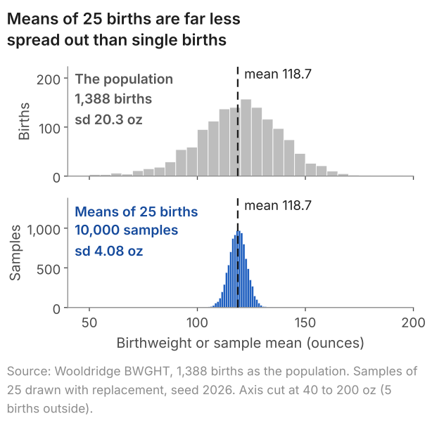
default_rng(2026), rng.choice(births, size=(10000, 25), replace=True), one row per sample.The top panel of Figure 1 is a histogram of the population; the bottom panel, on the same scale, of the 10,000 sample means. In this run the two share a centre, but the means are about a fifth as spread out and more symmetric, without the population's long tail of light babies, down to 23 ounces. The next sections take the centre, the spread and the shape in turn.
4. Where it is centred: the sample mean is unbiased
Is the sample mean right on average? Its average over all possible samples is its expectation, \(E[\bar X]\), and the question is whether that equals \(\mu\). Under random sampling each \(X_i\) is a draw from the population, so each has expectation \(\mu\); and the expectation of a sum is the sum of the expectations, with a constant multiplier taken outside (lesson 3). Hence
$$ \begin{aligned} E[\bar X] &= \frac{1}{n}\big(E[X_1] + \dots + E[X_n]\big) \\ &= \frac{1}{n}\, n\mu = \mu . \end{aligned} $$In words: averaged over all possible samples, the sample mean equals the population mean.
An estimator, a statistic used to estimate a parameter (here \(\bar X\) for \(\mu\)), is called unbiased if its expectation equals that parameter: across samples its misses above and below cancel. That does not make any one sample mean equal to \(\mu\): sample 1 missed by 1.90 ounces. The argument used only the expectation of each draw, not the shape of the population, the sample size or even independence, so the sample mean is unbiased for every \(n\) and every shape of population. In the simulations, for \(n\) = 2, 5, 25 and 100, the 10,000 sample means average 118.51, 118.63, 118.71 and 118.75 ounces. Ten thousand samples are themselves a sample, so these averages miss 118.70 slightly, by at most 0.19.
5. How spread out it is: the variance of the sample mean
Section 1's five samples missed \(\mu\) by between 0.54 and 7.14 ounces. To quantify this sampling variation we need one measure of the size of such misses across all possible samples. By section 4 their plain average is zero, so we square them first.
A variance is the average squared distance of a random variable from its own mean (lesson 3), and the mean of \(\bar X\) is \(\mu\). So the variance of the sample mean is the average squared distance between the sample mean and the population mean, taken over all the samples we could have drawn:
$$ \operatorname{Var}(\bar X) = E\big[(\bar X - \mu)^2\big] . $$Under random sampling, with \(\sigma^2\) the variance of one observation in the population, it is
$$ \operatorname{Var}(\bar X) = \frac{\sigma^2}{n} . $$In words: variance of the sample mean = variance of one observation divided by the number of observations.
Show where the formula comes from, and where independence is used
- Write the mean as a sum. \(\bar X = \frac{1}{n}(X_1 + \dots + X_n)\): the sum of the \(n\) observations, times \(1/n\).
- Take the constant out. A constant \(a\) multiplying a random variable multiplies its variance by \(a^2\) (lesson 3). Here \(a = 1/n\), so $$ \begin{aligned} &\operatorname{Var}(\bar X) \\ &= \frac{1}{n^2}\operatorname{Var}(X_1 + \dots + X_n) . \end{aligned} $$
- Use independence. The variance of a sum is the sum of the variances plus twice the covariance of every pair (lesson 3). Under random sampling the observations are independent, so every covariance is zero and the variance of the sum is the sum of the \(n\) variances. Positively correlated observations would make it larger.
- Use identical distributions. Each observation has variance \(\sigma^2\), so the sum has variance \(n\sigma^2\), and $$ \operatorname{Var}(\bar X) = \frac{n\sigma^2}{n^2} = \frac{\sigma^2}{n} . $$
Why divide by \(n\)? Intuitively, the larger the sample, the more closely it resembles the population it was drawn from, and so the less one sample can differ from another by chance. One birth can lie far from \(\mu\): the lightest weighed 23 ounces, 96 below it. In a mean, heavy and light babies largely offset one another: sample 1's births run from 89 to 146 ounces, up to 30 from \(\mu\), yet their mean is 1.90 from it. As \(n\) increases the random variation in the sample mean decreases, and \(\sigma^2/n\) falls towards zero.
Why the square root? A variance is an average of squared distances, so \(\sigma^2/n\) is in ounces squared. Taking the square root returns it to ounces, the units the data are measured in, so that it can be read as a typical distance between the sample mean and the population mean:
$$ \sqrt{\operatorname{Var}(\bar X)} = \frac{\sigma}{\sqrt{n}} . $$In words: standard deviation of the sample mean = population standard deviation divided by the square root of the sample size.
The births are the whole population here, so \(\sigma\) is computed with divisor 1,388, not 1,387, and is 20.347 ounces. For \(n = 25\), \(\sigma/\sqrt{n} = 20.347/5 = 4.07\) ounces: about 20 ounces for one birth, about 4 for a mean of 25.
The derivation used random sampling and a finite variance, and no particular \(n\) or shape of population. So the formula is exact for every \(n\); it is not a large-sample approximation. The table sets it beside the standard deviation of the 10,000 sample means in each simulation of section 4.
| Sample size n | 2 | 5 | 25 | 100 |
|---|---|---|---|---|
| \(\sigma/\sqrt{n}\), formula (oz) | 14.39 | 9.10 | 4.07 | 2.03 |
| Standard deviation of the 10,000 means (oz) | 14.27 | 9.19 | 4.08 | 2.04 |
The two rows agree to within about 1% at every \(n\), \(n = 2\) included. Since \(\sqrt{100}\) is twice \(\sqrt{25}\), four times the data halves the standard deviation of the sample mean, from 4.07 ounces at \(n = 25\) to 2.03 at \(n = 100\) (lesson 5). In practice \(\sigma\), a feature of the population, is unknown; replacing it by the sample standard deviation \(s\) gives the standard error of the mean, \(s/\sqrt{n}\), the subject of lesson 5.
6. The law of large numbers
Where the sample mean ends up as the sample keeps growing follows from sections 4 and 5. They give two facts under random sampling: \(\bar X\) is centred on \(\mu\) at every \(n\), and its variance \(\sigma^2/n\) falls towards zero as \(n\) grows, provided \(\sigma^2\) is finite. A random variable centred on \(\mu\) whose spread shrinks towards zero has less and less room to lie far from \(\mu\). Hence the law of large numbers: under random sampling from a population with finite variance, the probability that \(\bar X\) lies within any fixed distance \(\varepsilon\) of \(\mu\), however small, approaches 1 as \(n\) grows:
$$ P\big(|\bar X - \mu| \lt \varepsilon\big) \to 1 \ \text{ as } n \text{ grows}. $$In words: as the sample size increases, the sample mean becomes closer and closer to the population mean with increasing probability.
(A finite population mean is enough for the law itself; the argument above also uses the variance.) The law applies to the average of any quantity measured on independent draws whose mean is finite, not only to \(\bar X\). In a large sample the sample variance \(s^2\) is close to the average of the squared distances \((X_i - \mu)^2\), whose mean is \(\sigma^2\); so under random sampling \(s^2\) closes in on \(\sigma^2\), and \(s\) on \(\sigma\), as \(n\) grows. Section 7 shows the sample variance with divisor \(n\) doing so for simulated grades.
Figure 2 shows the law on simulated exam grades, normal with mean 65 and standard deviation 10. Each line is the running mean of one sequence of independent grades, the mean of the first \(n\), plotted against \(n\) on a log scale. The shaded band, \(65 \pm 1.96 \times 10/\sqrt{n}\), holds 95% of sample means of size \(n\).
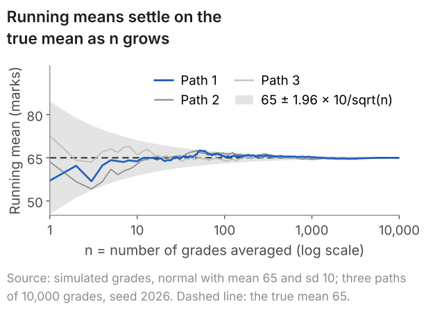
default_rng(2026), rng.normal(65, 10, size=(3, 10000)), one row per path, grades in the order drawn.After one grade the paths stand at 57.07, 63.61 and 72.69; as the band narrows, they close in on 65. The law is a statement about probability, so a running mean need not close in steadily, on real data as on simulated grades.
Show the law on real data: births and home wins
Drawing births at random one at a time, the running mean is 1.50 ounces below \(\mu\) after 10, 0.11 below after 100 and 1,000, and 0.22 below after 10,000.
A share is a mean too, of a variable that is 1 for a home win and 0 otherwise (lesson 3). In the 1,900 Premier League matches of 2019/20 to 2023/24 the share of home wins is 0.441; drawing matches at random, the running share is 0.700 after 10, 0.460 after 100, 0.461 after 1,000 and 0.4425 after 10,000.
The law is about the mean, not single observations: grade 10,000 is as likely to be far from 65 as grade 1 was. Nor is an early run above the mean made up later by a run below it: it is diluted. Independent draws have the same distribution whatever came before, so expecting a low draw after a run of high ones is a mistake, the gambler's fallacy.
Show the dilution in numbers: path 3 at n = 1,000
Path 3's first ten grades average 66.04, and grades 11 to 1,000 average 65.03, also above 65: no run below 65 makes up for the start. The first ten are a hundredth of the 1,000, so they carry weight 0.01 in the running mean at \(n = 1{,}000\):
$$ 0.01 \times 66.04 + 0.99 \times 65.03 = 65.04 . $$Their excess of 1.04 marks counts for 0.0104 of a mark at \(n = 1{,}000\): diluted, not repaid.
The reference page on the law of large numbers has an animation, the proof by Chebyshev's inequality and what happens with dependent data.
7. Unbiased and consistent are different properties
Sections 4 and 6 gave the sample mean two properties. Are they the same? An estimator is unbiased if its expectation equals the population value at every \(n\), and consistent if the probability that it lies within any fixed distance of that value approaches 1 as \(n\) grows. Two estimators, simulated in 100,000 samples of normal grades with mean 65 and variance 100, show that neither property implies the other.
- Unbiased, not consistent: the first observation alone. Its expectation is 65, the population mean, but its spread stays that of one grade: standard deviation 10.03 at \(n = 5\) and 9.96 at \(n = 100\). It lands within 1 mark of 65 in 7.8% and 7.9% of samples, against 17.7% and 68.5% for the sample mean: it does not close in on 65.
- Biased, consistent: the sample variance with divisor \(n\), not \(n - 1\). As lesson 3 shows, its expectation is \(100(n-1)/n\): 80 at \(n = 5\), 96 at 25, 99 at 100 and 99.8 at 500, too low on average. Its bias shrinks towards zero, and so does its spread (standard deviation 56.6 at \(n = 5\), 6.3 at \(n = 500\)), so it closes in on 100. The shrinking spread matters: the first observation has no bias at all, and it is not consistent.
8. The central limit theorem: the shape
Centre and spread do not give the probability that \(\bar X\) falls within a given distance of \(\mu\), which intervals and tests need. That takes the shape of the sampling distribution. A sum of independent normal random variables is itself normal, so under random sampling from a normal population \(\bar X\) is normal at every \(n\). The populations here are not normal.
As \(n\) grows the distribution of \(\bar X\) narrows onto \(\mu\), so a picture of \(\bar X\) itself hides its shape. To see the shape we measure the distance of \(\bar X\) from \(\mu\) in units of its standard deviation:
$$ Z = \frac{\bar X - \mu}{\sigma/\sqrt{n}} . $$In words: Z = (sample mean minus population mean) divided by the standard deviation of the sample mean.
Subtracting \(\mu\) moves the centre to 0 and dividing by \(\sigma/\sqrt{n}\) makes the standard deviation 1, as standardising does in lesson 2; the ounces cancel, so \(Z\) has no units. Sample 5 has \(z = (125.84 - 118.70)/4.07 = 1.75\). By sections 4 and 5, \(Z\) has mean 0 and standard deviation 1 at every \(n\), so only its shape can change with \(n\).
The central limit theorem
Under random sampling from a population with a finite variance, the distribution of \(Z\) is approximately standard normal in large samples, whatever the shape of the population. Equivalently, \(\bar X\) is approximately normal with mean \(\mu\) and variance \(\sigma^2/n\). As \(n\) grows, the error of the approximation goes to zero.
Remarks. The theorem is about the distribution of the sample mean across samples, not about the data: the population keeps its shape however large the sample.
Figure 3 tests it on a population nothing like a bell: an exponential population with mean 1 and standard deviation 1. It takes no negative values and has a long right tail, which pulls the mean up: 63% of its values lie below the mean. Each panel is a histogram of \(Z\) from 100,000 samples of one size, with the standard normal curve dashed and the values beyond ±1.96 in blue; the normal curve has 2.5% beyond each.
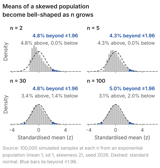
default_rng(2026) and rng.exponential(1.0, size=(100000, n)), one row per sample.A mean of two values that cannot be negative cannot lie more than 1.41 of its standard deviations below 1, so at \(n = 2\) nothing lies below -1.96. As \(n\) grows the histogram moves towards the curve, but the two tails even out slowly.
Real data show the same. Total goals in a match, with the 1,900 matches as the population, have mean 2.87 and standard deviation 1.68. They are skewed to the right: a match can fall at most 2.87 goals below the mean, yet 54 had 7 or more, over 4 above it. The first panel of Figure 4 is the population; the other three are histograms of the means of 100,000 samples of 5, 30 and 100 matches, each labelled with its standard deviation.
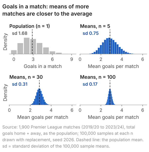
default_rng(2026) and rng.choice(goals, size=(100000, n), replace=True), one row per sample.The means narrow around 2.87 and lose the population's lopsided shape, while the matches themselves keep it, however large the sample.
Why does averaging produce a bell? (intuition, not proof)
An extreme mean needs the draws to be extreme together, which is unlikely, while a mean near the centre can come from a great number of mixtures of high and low draws. With two matches, a mean of 0 goals needs both to be goalless: probability \((107/1{,}900)^2 = 0.003\). A mean of 3 can come from seven pairs of totals (0 and 6, 1 and 5, 2 and 4, 3 and 3, and the first three reversed), with probability 0.161. The reference page works the same idea on a flat population.
The theorem also covers sums and shares (means of 0/1 variables), and versions of it cover other estimators built from sums, such as the regression slope of lesson 11. Lesson 6 combines it with the 1.96 of the normal distribution to build a confidence interval.
9. How large does n have to be?
How large \(n\) must be for the normal curve to be a good approximation depends on how skewed and heavy-tailed the population is, so there is no single number. Each cell of the table gives the percentages of 100,000 standardised sample means above +1.96 and below -1.96; the normal curve gives 2.5 and 2.5.
| Population | n = 5 | n = 30 | n = 100 |
|---|---|---|---|
| Births (slightly skewed to the left) | 2.2 and 2.8 | 2.5 and 2.7 | 2.4 and 2.5 |
| Goals in a match (skewed to the right) | 3.5 and 1.1 | 2.6 and 2.4 | 2.5 and 2.3 |
| Exponential (strongly skewed to the right) | 4.3 and 0.045 | 3.4 and 1.4 | 3.1 and 2.0 |
The births are close to 2.5 and 2.5 by \(n = 5\), the goals by \(n = 30\). The exponential is still lopsided at \(n = 30\), though its total, 4.8%, is close to 5%: the upper tail holds 3.4% and the lower 1.4%, where the normal curve gives 2.5% each. (These shares standardise with the population \(\sigma\). A test has to use \(s\) in its place, which changes the two tails again; the reference page shows by how much for skewed data.) So "n = 30 is enough" is a rule of thumb, not a guarantee.
Without a finite variance the theorem does not apply. In a Pareto population with mean 3 and infinite variance, 68% of 10,000 simulated sample means of size 10,000 lie below 3, where a normal curve centred on 3 would put 50%. The reference page explains this case and compares more populations.
10. Common mistakes
- "The sampling distribution is the distribution of the data." Single births have standard deviation 20.35 ounces; means of 25 births, 4.07.
- "Sample size does not change how much the mean varies." \(\sigma/\sqrt{n}\) is 14.39 ounces at \(n = 2\), 2.03 at \(n = 100\).
- "A skewed population gives a biased sample mean." Means of five exponential draws average 0.998 in 100,000 samples, against 1.
- "\(\sigma^2/n\) holds only in large samples." It is exact for every \(n\): at \(n = 2\), its square root \(\sigma/\sqrt{n}\) is 14.39 ounces against 14.27 simulated.
- Treating the sample mean as the population mean. Sample 1's 116.80 is a statistic; 118.70 is a parameter.
- Using the number of samples as \(n\). For 10,000 samples of 25 births, \(20.35/\sqrt{25} = 4.07\), not \(20.35/\sqrt{10{,}000} = 0.20\).
- "The central limit theorem makes the data normal." Goals in a match stay skewed; the mean of 30 matches is close to normal.
- "After a run above the mean, a run below is due." The gambler's fallacy: in path 3, grades 11 to 1,000 averaged 65.03, still above 65.
11. Check your understanding
Five questions, marked on the page; every option has an explanation, including the wrong ones. (Without JavaScript the explanations are shown beneath each question.)
1. Treat the 1,900 Premier League matches of 2019/20 to 2023/24 as the population: 838 of them, a share of 0.441, were home wins. A random sample of 100 of these matches contains 46 home wins, a share of 0.46. Which description is right?
It is tempting because 0.441 is also worked out from data. But those data are the whole population here, so 0.441 is the population share itself, a fixed number: a parameter. Only 0.46 depends on which 100 matches were drawn.
Correct. 0.441 describes the population and does not change. 0.46 was computed from one sample of 100 matches; another sample of 100 would give another share, scattered around 0.441.
Both are home-win shares, but only 0.441 describes the population. 0.46 comes from one sample of 100 matches and would change with the sample: it is a statistic, an estimate of 0.441.
2. From the 1,388 births (standard deviation 20.35 ounces), 10,000 samples of 25 births are drawn, and a histogram is made of the 10,000 sample means. Its standard deviation is 4.08 ounces. What does the histogram show?
Correct. Each value in the histogram is one sample's mean, so the histogram traces the sampling distribution of the mean of 25 births. Its standard deviation, 4.08 ounces, is close to σ/√n = 20.35/√25 = 4.07.
That is the distribution of the data, the 1,388 births, with standard deviation 20.35 ounces. The histogram holds means of samples of 25, which vary far less: 4.08 ounces.
That would be a histogram of 25 birthweights, such as sample 1's, which run from 89 to 146 ounces. This histogram has one value per sample, its mean, and shows how the 10,000 means vary.
3. Total goals in the 1,900 matches, taken as the population, have mean 2.87 and standard deviation 1.68. Under random sampling, what are the mean and the standard deviation of the sample mean for samples of 100 matches?
This divides the standard deviation by n: 1.68/100. It is the variance that is divided by n; the standard deviation is divided by √n = 10.
This is the variance of the sample mean, σ²/n = 1.68²/100 = 0.0282, in goals squared. The standard deviation is its square root, 0.168, back in goals.
Correct. The sample mean is centred on the population mean, 2.87, and its standard deviation is σ/√n = 1.68/√100 = 0.168 goals. The simulation behind Figure 4 gives 0.17.
1.68 is the standard deviation of a single match's goals. The mean of 100 matches varies far less: its standard deviation is 1.68/√100 = 0.168.
4. Grades are drawn independently from a normal population with mean 65 and standard deviation 10. In path 3 of Figure 2, the first grade is 72.69 and the first ten grades average 66.04. What can be said about grade 11?
This is the gambler's fallacy. With independent draws, grade 11 falls below 65 with probability 0.5, whatever came before. The early excess is not paid back: it is diluted, with weight 10/n in the running mean.
The law of large numbers is about the mean of a large number of grades, not single grades. Grade 11 still has standard deviation 10, and it lies within 7.69 of 65 with probability 0.56, the same as any single grade.
Correct. With independent draws, grade 11 is normal with mean 65 and standard deviation 10, like every other grade. The law of large numbers describes the running mean, not single grades.
5. For an exponential population (mean 1, standard deviation 1, a long right tail), the share of standardised sample means above +1.96 is 4.8% at n = 2, 3.4% at n = 30 and 3.1% at n = 100. Which statement explains the trend?
Correct. Under random sampling, with a finite variance, the central limit theorem says that the distribution of the standardised mean approaches the standard normal, which has 2.5% above +1.96. The shares move towards it: 4.8%, 3.4%, 3.1%.
The population does not change when more is drawn from it: it keeps its long right tail at every n. What changes is the distribution of the mean of n draws.
At n = 100 the sample mean still varies, with standard deviation 1/√100 = 0.1, so it does not equal 1. The shares describe the shape of its distribution, which approaches the normal.
12. Three questions about sampling distributions
A sampling distribution is the distribution of a statistic, such as the sample mean, over all the samples of a given size that could be drawn. It is not the distribution of the data. Single birthweights have a standard deviation of 20.35 ounces; means of 25 births have a sampling distribution with standard deviation 4.07 ounces.
The law of large numbers says where the sample mean ends up: under random sampling it closes in on the population mean as n grows. The central limit theorem gives the shape of its distribution: with random sampling and a finite variance, approximately normal in large samples, with standard deviation σ/√n. For means of 100 births that is 2.03 ounces.
There is no single number: it depends on how skewed the population is. Means of birthweights, a nearly symmetric population, are close to normal by n = 5. For a strongly skewed exponential population, at n = 30 3.4% of standardised means still lie above +1.96 and 1.4% below, against 2.5% each. Thirty is a rule of thumb.
13. Where next
- Lesson 5: standard deviation versus standard error: \(s\) in place of \(\sigma\) gives \(s/\sqrt{n}\), the standard error that software prints.
- Lesson 6: confidence intervals, built on the central limit theorem.
- The reference pages on the law of large numbers and the central limit theorem: animations, Chebyshev's inequality, dependent data and more populations.
- Lesson 3: expectation, variance, covariance and correlation (previous) and the course home, which lists all 25 lessons and says which are published.
Unsure what is random and what is fixed? Send the question
I tutor statistics and econometrics one-to-one, from a first sampling distribution through to regression, panel data and time series. Bring the question you are stuck on and we will work through it in the free 30-minute consultation.
Book a free 30-minute consultation Econometrics tutor: how it works
Data and simulation. Births: Wooldridge, Introductory Econometrics: A Modern Approach, data set BWGHT (1,388 births, 1988 National Health Interview Survey), treated as the population in this lesson; results quoted, data not republished. Matches: openfootball/england (CC0), the 1,900 Premier League matches of 2019/20 to 2023/24 in file order, treated as a population; goals is home plus away goals and home_win is 1 if the home side won, 0 otherwise. Each simulation starts from its own fresh numpy default_rng(2026) and draws one array, one row per sample, filled row by row in the order drawn; births and matches are drawn with replacement. Section 1: rng.choice(births, size=(5, 25), replace=True). Sections 3 to 5: rng.choice(births, size=(10000, n), replace=True) for n = 2, 5, 25 and 100. Section 6: rng.normal(65, 10, size=(3, 10000)); rng.choice(births, size=10000, replace=True); from a second fresh generator, rng.choice(home_win, size=10000, replace=True). Section 7: rng.normal(65, 10, size=(100000, n)) for each n. Sections 8 and 9: rng.exponential(1.0, size=(100000, n)), rng.choice(goals, size=(100000, n), replace=True) and rng.choice(births, size=(100000, n), replace=True) for each n; Pareto, 1 + rng.pareto(1.5, size=(10000, 10000)). Standardised means use the population mean and the population standard deviation (divisor N). Adapted from my lecture notes for the MSc pre-sessional statistics course (ECON60901, 2015 and 2016) and for Time Series Econometrics (ECON30401) at the University of Manchester, and for Financial Econometrics (EC5609) at the University of St Andrews.