
To learn about a process from one observed history, the process must behave the same way throughout the sample. Stationarity is that requirement: a constant mean and variance, and dependence that varies only with the gap between dates. A random walk breaks it, and regressing one random walk on an unrelated one can report a relationship that is not there.
In this lesson
- Why one history needs a stable process
- Stationarity: what stays the same
- Looking for it in data: a sample in two halves
- White noise: no autocorrelation at all
- The random walk: every shock kept
- Differences: from a random walk back to its shocks
- Spurious regression: two unrelated random walks
- What to do with a trending series
- Common mistakes
- Check your understanding: five marked questions
- Four questions about stationarity and random walks
- Where next
1. Why one history needs a stable process
Every summary of a time series pools observations from different dates. Over the 144 quarters from 1984 Q1 to 2019 Q4, UK GDP grew by 0.56% a quarter on average, with a standard deviation of 0.64 percentage points (ONS figures as published in September 2026). The quarters from 2020 are left out, because two pandemic quarters would dominate every statistic (lesson 22). Reading 0.56 as an estimate of the mean of the process presumes that there is one mean, shared by every quarter.
Take the extreme case where the distribution of \(Y_t\), the process at date \(t\), is different in every quarter. (As in lesson 21, the capital \(Y_t\) is the process and \(y_1, \dots, y_T\) are the \(T\) values observed.) Each quarter then has its own mean and variance, and of each distribution we hold one observation. One observation says next to nothing about the spread of the distribution it came from, and the average of 144 quarters mixes 144 different means into a number that estimates none of them. \(T\) observations tell us more than one only if their distributions share something.
Stationarity is the assumption that they share their mean, their variance and the way each value depends on earlier ones. Add that the dependence between distant dates dies away, so that a longer history carries more information (lesson 21 shows how much less positively correlated observations carry), and 0.56 estimates the mean of the process and 0.64 its standard deviation.
What students say
“Nicky is an excellent econometrics tutor. He explains complex concepts clearly and makes them much easier to understand.”
“I was completely lost in my economics class, and then I started working Nicky and he totally saved me. He was excellent at explaining the material and extremely accommodating to meet with me many times despite us being in different time zones! Highly recommend working with Nicky!”
“Nicky is a very good and thorough teacher. He has excellent knowledge of econometrics and takes the time to work through your questions. Highly recommended!”
“Really great tutor! Encouraging, knowledgeable, friendly”
“Very good lesson, Nicky is very helpful.”
“Very helpful and clear.”
“I gather it was very useful, thank you!”
“Fantastic!”
2. Stationarity: what stays the same
The definition turns "behaves the same way" into three conditions. In it, \(E[Y_t]\) is the mean of \(Y_t\) across all the histories the process could produce, taken at one date \(t\) (lesson 21), not an average over dates. \(\gamma(k)\) is the autocovariance at lag \(k\), the covariance of two values \(k\) periods apart (lesson 23), and \(\gamma(0)\) is the variance.
Definition: stationarity
A process \(Y_t\) is stationary if, at every date \(t\),
$$ \begin{aligned} E[Y_t] &= \mu , \\ \operatorname{Var}(Y_t) &= \gamma(0) < \infty , \\ \operatorname{Cov}(Y_t, Y_{t-k}) &= \gamma(k) , \end{aligned} $$for each lag \(k = 1, 2, \dots\), where the mean \(\mu\), the variance \(\gamma(0)\) and the autocovariances \(\gamma(k)\) are numbers that do not depend on \(t\).
Remarks. Intuitively, if a process is stationary its distribution remains the same over time: it does not move or change, hence the name. Strictly, the definition fixes only the mean, the variance and the autocovariances, so it is also called weak or covariance stationarity; strict stationarity, which fixes the whole distribution, is not needed here. Stationarity is a property of the process, and data can only look consistent with it or not. Stationary does NOT mean "no trend": a process whose variance grows is not stationary even if its mean never moves, as with the random walk of section 5.
Each condition rules out one kind of change. The first rules out a drifting mean: UK real GDP was 4.98 times as large in 2026 Q2 as in 1955 Q1 (lesson 22). The second rules out a changing spread: IBM's monthly returns had a standard deviation of 4.9% in 1936 to 1945 and 10.6% in 1996 to 2003 (lesson 22). Data like these are hard to reconcile with a constant mean or a constant variance. The third makes the link between two values depend only on how far apart they are, so the correlation between growth in one quarter and the next, \(\rho(1) = \gamma(1)/\gamma(0)\), is the same in 1990 as in 2015. That is what lets lesson 23 estimate one autocorrelation per lag from a whole sample.
Stationarity is only an assumption, and it may not hold. Books use other letters (some write \(\sigma^2\) for the variance of \(Y_t\); here \(\sigma^2\) is kept for the shocks), and the choice is cosmetic.
3. Looking for it in data: a sample in two halves
Stationarity cannot be read off one history, but a history can look inconsistent with it. The simplest check splits the sample in two and compares the means and standard deviations of the halves, which under stationarity differ only by chance.
| Series | Mean, first half | Mean, second half | Std. dev., first half | Std. dev., second half |
|---|---|---|---|---|
| UK GDP growth, % a quarter | 0.688 | 0.434 | 0.655 | 0.606 |
| Log of UK real GDP (£ million) | 12.906 | 13.306 | 0.134 | 0.083 |
| IBM monthly returns, % | 1.79 | 1.04 | 6.85 | 7.34 |
Halves: 1984 Q1 to 2001 Q4 and 2002 Q1 to 2019 Q4 for the GDP series (72 quarters each); January 1926 to December 1964 and January 1965 to December 2003 for IBM (468 months each).
The log of real GDP fails the check plainly. Its mean is 0.400 higher in the second half, so GDP there is about \(e^{0.400} = 1.49\) times as high on a geometric average, and its standard deviation within each half measures the climb inside the half, not a stable spread. GDP growth has a similar spread in the two halves, but its mean fell from 0.688% to 0.434% a quarter, which lesson 22 reads as a possible shift in the mean. Whether a fall of 0.25 percentage points is more than chance the table cannot say: growth is persistent (\(r(1) = 0.556\)), and the means of two halves of one persistent history can differ by chance (lesson 21). IBM's halves differ little next to the spread of the returns: their means differ by about a tenth of the standard deviation of 7.11. Yet decade by decade the standard deviation ran from 4.9 to 10.6, so halves can hide changes within them.
A clear difference between halves is evidence against a constant mean or variance, but agreement does not establish stationarity: the process can change within each half, and the split says nothing about the third condition. Judging how large a difference chance can produce needs a test, which this lesson does not cover.
4. White noise: no autocorrelation at all
The simplest stationary process has no dependence between dates that a correlation can detect. It is called white noise, and the shocks \(\varepsilon_t\) of every model in this part of the course are white noise.
Definition: white noise
A process \(Y_t\) is white noise if, at every date \(t\),
$$ \begin{aligned} E[Y_t] &= 0 , \\ \operatorname{Var}(Y_t) &= \sigma^2 < \infty , \\ \operatorname{Cov}(Y_t, Y_{t-k}) &= 0 , \end{aligned} $$for each lag \(k = 1, 2, \dots\). For short we write \(Y_t \sim \text{WN}(\sigma^2)\).
Remarks. Intuitively, white noise fluctuates around zero with a constant spread, and no straight-line rule in past values predicts the next value better than its mean, zero. If \(Y_t\) is independent and identically distributed with mean zero and finite variance, it is white noise; if it is white noise, it is stationary. Neither statement reverses, and white noise need not be normal. Stationarity and white noise are NOT the same thing: a stationary process may have autocovariances that are not zero, provided they stay the same over time.
Stationary but not white noise: a stationary AR(1) with \(\phi = 0.5\), which has autocorrelation 0.5 at lag 1. White noise but not independent: IBM's monthly returns look like this (Figure 1).
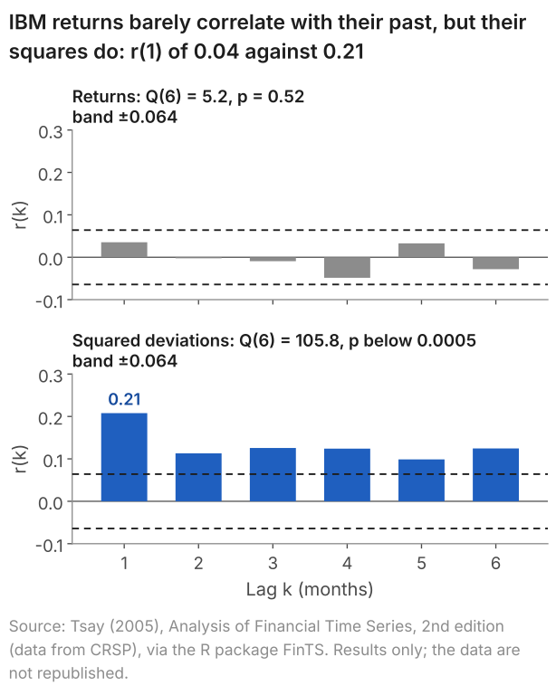
In the top panel every bar lies inside the band \(\pm 0.064\), the approximate 95% range that lesson 23 builds for the sample autocorrelation \(r(k)\) when the observations are independent, and the Ljung-Box test of the six lags together gives \(p = 0.515\). Less their mean of 1.42% a month, the returns are consistent with white noise at these lags. The bottom panel is for the squared deviations from that mean, which measure the size of each month's move whatever its sign. All six bars lie outside the band, with \(r(1) = 0.208\) and a p-value below 0.0005: large moves of either sign come in clusters (lesson 22). The size of one month's return is correlated with the size of the last, though the return itself shows no sign of autocorrelation, so the data are evidence that the returns are not independent. Autocorrelation detects linear dependence only, and white noise asks for nothing more than its absence.
5. The random walk: every shock kept
A much studied way for a process to fail stationarity is the random walk. Each period it adds a new shock to the previous value and keeps it:
$$ Y_t = Y_{t-1} + \varepsilon_t , $$where \(\varepsilon_t\) is white noise with variance \(\sigma^2\). It is the AR(1) of lesson 25, \(Y_t = \alpha + \phi Y_{t-1} + \varepsilon_t\), with \(\alpha = 0\) and \(\phi = 1\).
In words: this period's value = last period's value + a new shock.
To judge it against the definition we need its mean and variance at each date. From a fixed start \(Y_0\), substituting back gives \(Y_t = Y_0 + \varepsilon_1 + \dots + \varepsilon_t\): the start plus every shock so far. The shocks have mean zero, so \(E[Y_t] = Y_0\) at every date, and the mean does not move. White-noise shocks are uncorrelated, so their variances add:
$$ \operatorname{Var}(Y_t) = t\sigma^2 . $$In words: variance at date t = number of shocks so far × variance of one shock.
Show where \(t\sigma^2\) comes from
- Substitute back to the start. \(Y_t = Y_{t-1} + \varepsilon_t\), \(Y_{t-1} = Y_{t-2} + \varepsilon_{t-1}\), and so on down to \(Y_1 = Y_0 + \varepsilon_1\). Putting each into the one above, $$ Y_t = Y_0 + \varepsilon_1 + \varepsilon_2 + \dots + \varepsilon_t . $$
- Drop the start. \(Y_0\) is a fixed number, and adding a constant does not change a variance, so \(\operatorname{Var}(Y_t) = \operatorname{Var}(\varepsilon_1 + \dots + \varepsilon_t)\).
- Add the variances. The variance of a sum is the sum of the variances plus twice every covariance. White-noise shocks are uncorrelated, so every covariance is zero, and \(t\) shocks of variance \(\sigma^2\) give \(t\sigma^2\).
The rule for the variance of a sum is in lesson 3. The same substitution gives the autocovariance: \(Y_t\) and \(Y_{t-k}\) share the first \(t - k\) shocks, so \(\operatorname{Cov}(Y_t, Y_{t-k}) = (t-k)\sigma^2\), which also depends on \(t\).
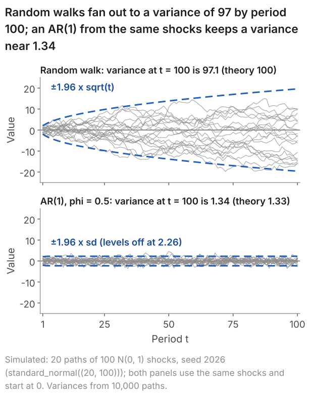
Intuitively, a random walk forgets nothing: each new shock is added in full and none fades, so the variance gains \(\sigma^2\) every period. An AR(1) with \(\phi = 0.5\) keeps half of the previous value, and so a quarter of its variance, before adding a shock. Its variance settles where what is lost equals what is added, at \(\sigma^2/(1 - 0.5^2) = 1.333\sigma^2\): the variance \(\sigma^2/(1 - \phi^2)\) of a stationary AR(1) (\(|\phi| < 1\), run from the distant past), which lesson 25 derives. With \(\phi = 1\) nothing is lost, so nothing settles. The variance is in the squared units of \(Y_t\); its square root, \(\sigma\sqrt{t}\), is the typical distance from the start in the units of \(Y_t\), ten times one shock's standard deviation after 100 periods.
So the variance of a random walk is finite at every date but grows without limit, and the process is not stationary, although its mean never moves. Nor is it explosive, a word kept for \(|\phi| > 1\), where each value is the last multiplied by more than one in size. The random walk is the simplest process with a unit root, the general name for nonstationarity of this kind; tests for one are beyond this lesson.
Figure 2 shows \(t\sigma^2\) at work, with \(\sigma = 1\): random walks, and AR(1) paths with \(\phi = 0.5\) built from the same shocks.
| Period t | Random walk: variance | Theory, \(t\sigma^2\) | AR(1), \(\phi = 0.5\): variance | Theory |
|---|---|---|---|---|
| 25 | 24.54 | 25 | 1.342 | 1.333 |
| 50 | 49.17 | 50 | 1.335 | 1.333 |
| 100 | 97.07 | 100 | 1.337 | 1.333 |
The table gives the variances across all 10,000 paths. The random walks' variance grows in step with \(t\). At \(t = 100\) it is 97.07 in this run, 2.9 below 100: about two simulation standard errors (a variance estimated from 10,000 such paths has a standard error of 1.41), a chance shortfall. The AR(1)'s variance stays near 1.333 at all three dates. Started at 0, the AR(1) moves towards its stationary distribution: its variance is 1 at \(t = 1\) and equals 1.333 to three decimals from \(t = 6\) on.
6. Differences: from a random walk back to its shocks
A random walk is the sum of its shocks, so the change from one period to the next is the latest shock. The first difference of \(Y_t\), written \(\Delta Y_t\), is that change:
$$ \Delta Y_t = Y_t - Y_{t-1} = \varepsilon_t . $$In words: the change in a random walk = this period's shock.
So the level of a random walk is not stationary, but its first difference is white noise, which is. Figure 3 shows one simulated random walk of 200 periods and its 199 changes.
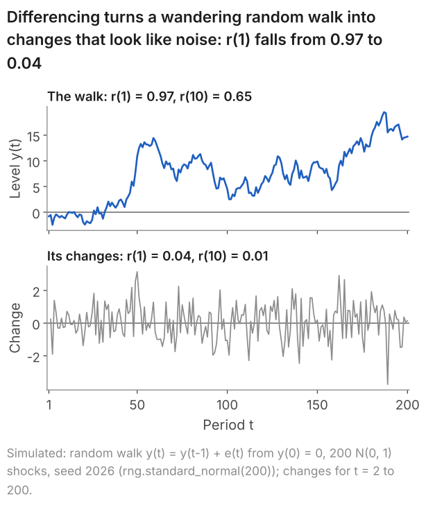
The level wanders far from its start and stays highly autocorrelated even ten periods apart (\(r(10) = 0.649\)): \(Y_t\) and \(Y_{t-k}\) share the first \(t - k\) shocks, so the level stays close to where it was. The changes share no shocks. One of their first ten autocorrelations, \(r(4) = -0.167\), lies outside the band ±0.139. Independent data produce such bars too: at least one of twelve falls outside in 40% of series of 144 independent values (lesson 23).
Log real GDP shows the same contrast between level and difference. The table gives the sample autocorrelations of its level over the 144 quarters from 1984 Q1 to 2019 Q4, of its first difference (100 times the change in the log) and of percentage growth.
| Lag k | Log real GDP, level | 100 × change in log GDP | Growth, % |
|---|---|---|---|
| 1 | 0.978 | 0.558 | 0.556 |
| 2 | 0.955 | 0.416 | 0.416 |
| 3 | 0.931 | 0.236 | 0.237 |
| 4 | 0.908 | 0.042 | 0.042 |
The level's autocorrelations are near 1 and fall slowly, the shape lesson 23 shows for a trending level; those of the difference lie outside the band ±0.163 at lags 1 to 3 and then drop close to zero. The first difference of the log is almost the growth rate: in these quarters \(100(\ln \text{GDP}_t - \ln \text{GDP}_{t-1})\) and \(100(\text{GDP}_t/\text{GDP}_{t-1} - 1)\) never differ by more than 0.031 percentage points. So studying growth, as lesson 22 does for a trending level, is studying the first difference of the log. Whether log GDP itself is a random walk with drift, which adds a constant \(\alpha\) each period as well as a shock, this lesson leaves open (section 8).
7. Spurious regression: two unrelated random walks
Two random walks that have nothing to do with each other show what nonstationarity does to a regression. We simulate two random walks of 100 periods, \(X_t\) and \(Y_t\), each starting at 0 with its own independent N(0, 1) shocks. We fit \(Y_t = \beta_0 + \beta_1 X_t + u_t\) by OLS, where \(u_t\) is the regression error, and test \(H_0: \beta_1 = 0\) (no relationship) with the usual t-test at the 5% level (lesson 7). Here \(H_0\) is true by construction. Figure 4 shows the first pair.
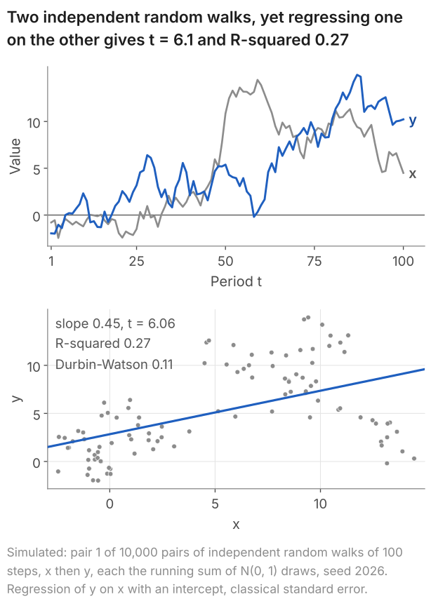
The table gives this pair's regression in levels and in changes, with the slope, standard error and t to the digits that R prints.
| Regression | Slope | Std. error | t | R-squared | Durbin-Watson |
|---|---|---|---|---|---|
| Levels: \(y_t\) on \(x_t\), 100 periods | 0.45233 | 0.07469 | 6.056 | 0.272 | 0.112 |
| Changes: \(\Delta y_t\) on \(\Delta x_t\), 99 periods | -0.1181 | 0.1135 | -1.041 | 0.011 | 2.061 |
R: the code
# two independent random walks, 100 periods: y on x, then the changes in y on the changes in x
walks <- read.csv("two-random-walks.csv")
summary(lm(y ~ x, data = walks))
summary(lm(diff(y) ~ diff(x), data = walks))
R: what it prints
> # two independent random walks, 100 periods: y on x, then the changes in y on the changes in x
> walks <- read.csv("two-random-walks.csv")
> summary(lm(y ~ x, data = walks))

Call:
lm(formula = y ~ x, data = walks)

Residuals:
    Min      1Q  Median      3Q     Max
-9.0680 -2.5523 -0.1536  2.8923  7.8840

Coefficients:
            Estimate Std. Error t value Pr(>|t|)
(Intercept)  2.83938    0.54182   5.240 9.20e-07 ***
x            0.45233    0.07469   6.056 2.58e-08 ***
---
Signif. codes:  0 ‘***’ 0.001 ‘**’ 0.01 ‘*’ 0.05 ‘.’ 0.1 ‘ ’ 1

Residual standard error: 3.855 on 98 degrees of freedom
Multiple R-squared:  0.2724,	Adjusted R-squared:  0.2649
F-statistic: 36.68 on 1 and 98 DF,  p-value: 2.575e-08

> summary(lm(diff(y) ~ diff(x), data = walks))

Call:
lm(formula = diff(y) ~ diff(x), data = walks)

Residuals:
    Min      1Q  Median      3Q     Max
-3.9776 -0.7765  0.0660  0.6819  2.6702

Coefficients:
            Estimate Std. Error t value Pr(>|t|)
(Intercept)   0.1294     0.1159   1.116    0.267
diff(x)      -0.1181     0.1135  -1.041    0.300

Residual standard error: 1.152 on 97 degrees of freedom
Multiple R-squared:  0.01105,	Adjusted R-squared:  0.0008578
F-statistic: 1.084 on 1 and 97 DF,  p-value: 0.3004
Python: the code
import pandas as pd
import statsmodels.formula.api as smf

# two independent random walks, 100 periods: y on x, then the changes in y on the changes in x
walks = pd.read_csv("two-random-walks.csv")
levels = smf.ols("y ~ x", data=walks).fit()
print(levels.summary())
walks["dx"] = walks["x"].diff()  # change from the period before (none for t = 1)
walks["dy"] = walks["y"].diff()
changes = smf.ols("dy ~ dx", data=walks).fit()
print(changes.summary())
Python: what it prints
                            OLS Regression Results
==============================================================================
Dep. Variable:                      y   R-squared:                       0.272
Model:                            OLS   Adj. R-squared:                  0.265
Method:                 Least Squares   F-statistic:                     36.68
Date:                Sat, 10 Oct 2026   Prob (F-statistic):           2.58e-08
Time:                        21:43:29   Log-Likelihood:                -275.83
No. Observations:                 100   AIC:                             555.7
Df Residuals:                      98   BIC:                             560.9
Df Model:                           1
Covariance Type:            nonrobust
==============================================================================
                 coef    std err          t      P>|t|      [0.025      0.975]
------------------------------------------------------------------------------
Intercept      2.8394      0.542      5.240      0.000       1.764       3.915
x              0.4523      0.075      6.056      0.000       0.304       0.601
==============================================================================
Omnibus:                        0.539   Durbin-Watson:                   0.112
Prob(Omnibus):                  0.764   Jarque-Bera (JB):                0.658
Skew:                          -0.009   Prob(JB):                        0.720
Kurtosis:                       2.603   Cond. No.                         10.3
==============================================================================

Notes:
[1] Standard Errors assume that the covariance matrix of the errors is correctly specified.
                            OLS Regression Results
==============================================================================
Dep. Variable:                     dy   R-squared:                       0.011
Model:                            OLS   Adj. R-squared:                  0.001
Method:                 Least Squares   F-statistic:                     1.084
Date:                Sat, 10 Oct 2026   Prob (F-statistic):              0.300
Time:                        21:43:29   Log-Likelihood:                -153.44
No. Observations:                  99   AIC:                             310.9
Df Residuals:                      97   BIC:                             316.1
Df Model:                           1
Covariance Type:            nonrobust
==============================================================================
                 coef    std err          t      P>|t|      [0.025      0.975]
------------------------------------------------------------------------------
Intercept      0.1294      0.116      1.116      0.267      -0.101       0.359
dx            -0.1181      0.113     -1.041      0.300      -0.343       0.107
==============================================================================
Omnibus:                        5.687   Durbin-Watson:                   2.061
Prob(Omnibus):                  0.058   Jarque-Bera (JB):                5.121
Skew:                          -0.456   Prob(JB):                       0.0773
Kurtosis:                       3.640   Cond. No.                         1.06
==============================================================================

Notes:
[1] Standard Errors assume that the covariance matrix of the errors is correctly specified.
The code reads two-random-walks.csv (100 rows: t, x, y), the pair in Figure 4. Save it in your working folder first. Python also prints the Durbin-Watson statistic; R does not.
In levels \(t = 6.06\) and the p-value is below 0.0005: the test rejects \(\beta_1 = 0\) firmly, and R-squared says that \(x_t\) accounts for 27% of the variation in \(y_t\). In changes \(t = -1.04\) and \(p = 0.300\): no evidence of a relationship. We built the data, so we know the second verdict is right.
One pair could be bad luck, so we repeat the experiment 10,000 times at each of three lengths. Figure 5 shows the share of pairs with a slope "significant at 5%", meaning \(|t| > 1.96\).
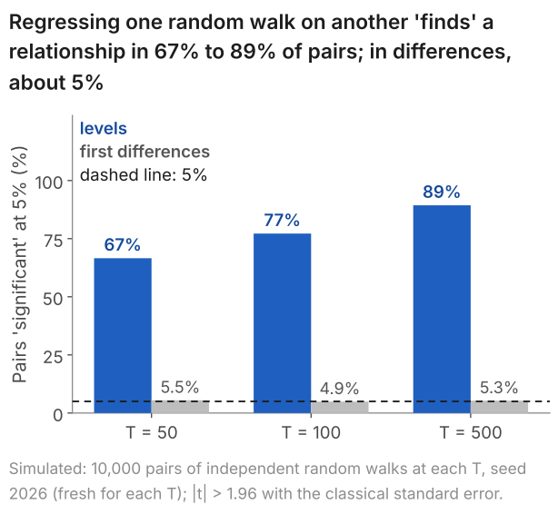
In levels the test rejects a true null hypothesis in 66.6%, 77.2% and 89.3% of pairs at \(T = 50\), 100 and 500, where a 5% test should reject in about 5%: more data make it worse. In changes it rejects in 5.5%, 4.9% and 5.3% of pairs, each within two simulation standard errors (0.2 points) of the exact rate for the cut-off 1.96 at that sample size (5.6%, 5.3% and 5.1%).
The 5% rests on assumptions about the regression error. Lesson 11 derives the standard error of the slope for errors that are independent of each other with the same variance at every observation. Under \(H_0\) the model is \(Y_t = \beta_0 + u_t\), so \(u_t = Y_t - \beta_0\) is the random walk \(Y_t\) shifted by a constant, and both assumptions fail. Its variance grows with \(t\), and \(u_t\) and \(u_{t-1}\) share all but the latest shock, so neighbouring errors are nearly equal: pair 1's residuals have \(r(1) = 0.927\) and a Durbin-Watson statistic of 0.112, where independent errors give about 2. The formula counts 100 errors as 100 independent pieces of information about the slope. Errors and a regressor that both move in long swings carry far fewer (lesson 21), so the formula understates how far the estimated slope \(\hat\beta_1\) strays from zero: across the 10,000 pairs of 100 periods the slopes have a standard deviation of 0.62, but the standard error averages 0.10. Hence \(t\), the slope divided by that standard error, comes out far too large.
More data do not help. The slopes are as spread out at \(T = 500\) as at \(T = 50\), with a standard deviation of 0.62 or 0.63, while the average standard error falls from 0.15 to 0.04 as if each period added independent information; so the median \(|t|\) rises from 3.11 to 10.07. In changes the two agree: at \(T = 100\) both are 0.102.
This is spurious regression, demonstrated by Granger and Newbold (1974): a regression between nonstationary series that reports a relationship where none exists. Its cause is the failure of the test's assumptions, with both series nonstationary and the error itself a random walk; it is not that the two walks happen to be correlated. Sizeable sample correlations are what unrelated random walks produce: at \(T = 100\) the mean R-squared is 0.24 and 16.0% of pairs exceed 0.5, and at \(T = 500\) the mean is still 0.237. The t-test, built for independent errors, reads them as evidence. The R-squared explainer uses the same pairs at \(T = 100\).
Real series show the same warning signs. Regress the log of UK real GDP on the log of the consumer prices index for the 128 quarters from 1988 Q1 to 2019 Q4, over which both climb. In levels the slope is 0.898 with \(t = 35.5\) and R-squared 0.909, but the residuals have \(r(1) = 0.976\) and a Durbin-Watson statistic of 0.025, the pattern of Figure 4. In quarterly growth rates, 100 times the change in each log (127 quarters), the slope is -0.174 with \(t = -2.38\) and R-squared 0.043, and the residuals still have \(r(1) = 0.611\), so this t is not reliable either. Neither regression is a model of output or prices, and neither settles whether the two are related; together they show that an R-squared of 0.91 between trending series says almost nothing, and that residuals deserve a look before a t-statistic is believed.
8. What to do with a trending series
For a series that trends or wanders, such as the level of GDP or of prices, the starting point is its changes: first differences, or growth rates, which are almost the first differences of the logs (section 6). In changes the t-test of section 7 rejected in about 5% of pairs, as it should. Differencing is not a cure for every case, though. When two nonstationary series do share a long-run relationship, which is called cointegration, differencing discards that relationship, and handling it is beyond this lesson. Nor is every trend a random walk with drift: a series can be a fixed line plus stationary deviations that return to the line after each shock, whereas a random walk with drift keeps every shock, and over one sample the two can look alike.
9. Common mistakes
- "Stationary means no trend." A random walk's mean stays at its start, yet its variance, \(t\sigma^2\), grows: it is not stationary.
- "The data are stationary." Stationarity belongs to the process; data look consistent with it or not. The log of GDP, whose mean climbs by 0.400 between the halves, does not.
- Treating white noise and stationarity as the same thing. A stationary AR(1) with \(\phi = 0.5\) has autocorrelation 0.5 at lag 1, not 0.
- "White noise means independent." IBM's returns have \(r(1) = 0.035\), but their squared deviations have \(r(1) = 0.208\): consistent with white noise, not with independence.
- Calling a random walk explosive, or its variance infinite. Its variance, \(t\sigma^2\), is finite at every date and grows without limit; "explosive" means \(|\phi| > 1\).
- Reading a large t between two trending series as a relationship. Between two unrelated random walks of 100 periods, \(|t| > 1.96\) in 77% of 10,000 pairs.
10. Check your understanding
Five questions, marked on the page; every option has an explanation, including the wrong ones. (Without JavaScript the explanations are shown beneath each question.)
1. Suppose the process behind IBM's monthly returns has a mean of 1.42% at every date and no autocorrelation at any lag, but a standard deviation of 4.9% in 1936 to 1945 and 10.6% in 1996 to 2003. Is it stationary?
A constant mean is only the first of three conditions. The variance must also be the same at every date, and here it is 4.9² = 24.0 in 1936 to 1945 and 10.6² = 112.4 in 1996 to 2003.
Correct. Stationarity needs a constant mean, a constant finite variance and autocovariances that depend on the lag only. The mean and the autocovariances (all zero) pass; the variance, 4.9² = 24.0 in 1936 to 1945 against 10.6² = 112.4 in 1996 to 2003, does not.
White noise also needs a constant variance (and a mean of zero). With no autocorrelation but a variance that changes, the process is neither white noise nor stationary.
2. For IBM's monthly returns, January 1926 to December 2003 (936 months), r(1) to r(6) all lie inside the band ±0.064, with r(1) = 0.035. For their squared deviations from the mean, all six lie outside it, with r(1) = 0.208. What do the two correlograms show together?
Near-zero autocorrelations speak only to linear dependence. The squared deviations, with r(1) = 0.208 far outside ±0.064, show that the size of one month's move is related to the size of the last: evidence that the returns are not independent.
White noise asks only for mean zero, a constant variance and zero autocorrelation. The returns' own autocorrelations are all inside the band, so, less their mean, they are consistent with white noise; the dependence in the squares is dependence that white noise allows.
Correct. The returns show no sign of autocorrelation (r(1) = 0.035, all six lags inside ±0.064), so less their mean they are consistent with white noise. Their squared deviations do show it (r(1) = 0.208, all six lags outside): large moves of either sign follow large moves, a dependence that autocorrelation does not detect.
3. A random walk \(Y_t = Y_{t-1} + \varepsilon_t\) starts at \(Y_0 = 0\), and its shocks are white noise with standard deviation 2. What is the variance of \(Y_t\) at \(t = 25\)?
4 is the variance of one shock, 2². That would be the variance at every date for white noise; a random walk keeps every shock, so at t = 25 the variance is 25 × 4 = 100.
10 = 2 × √25 is the standard deviation of \(Y_{25}\), \(\sigma\sqrt{t}\). The variance is its square, 10² = 100.
50 = 25 × 2 multiplies the shocks' standard deviation by t. Variances add, not standard deviations: 25 shocks of variance 2² = 4 give 25 × 4 = 100.
Correct. From \(Y_0 = 0\), \(Y_{25} = \varepsilon_1 + \dots + \varepsilon_{25}\). The shocks are uncorrelated, so their variances add: 25 × 2² = 100. The standard deviation is √100 = 10.
4. A simulation draws 10,000 pairs of independent random walks of 100 periods and regresses y on x in each pair. The slope has |t| > 1.96 in 77% of the pairs. What is the 77%?
Correct. In every pair y is unrelated to x, so \(H_0: \beta_1 = 0\) is true, and a test working as designed would reject it in about 5% of pairs. It rejects in 77% because the regression error is a random walk, which breaks the assumptions behind the standard error.
The pairs are unrelated by construction, so they are related in none of them. The 77% is the share of pairs in which the test wrongly rejects \(\beta_1 = 0\), not a probability that the null hypothesis is false.
That is R-squared, a different number: its mean across the 10,000 pairs is 0.24. The 77% counts the pairs with |t| > 1.96.
5. A random walk \(Y_t = Y_{t-1} + \varepsilon_t\), with \(\varepsilon_t\) white noise of variance \(\sigma^2\), starts at \(Y_0 = 0\). Its mean is 0 at every date: it has no drift. Is it stationary?
A constant mean is one of three conditions. From a fixed start the variance of a random walk is \(t\sigma^2\), which grows with t, so the second condition fails.
Correct. \(Y_t = \varepsilon_1 + \dots + \varepsilon_t\), and the variances of uncorrelated shocks add, so \(\operatorname{Var}(Y_t) = t\sigma^2\): \(\sigma^2\) at t = 1 and \(100\sigma^2\) at t = 100. A constant mean does not make up for a variance that changes.
From a fixed start the variance at date t is \(t\sigma^2\), a finite number at every date. The random walk is not stationary because that number changes with t, growing without limit.
11. Four questions about stationarity and random walks
A time series is called stationary when the process behind it has a constant mean, a constant finite variance, and covariances that depend only on the gap between dates. Data can only look consistent with it: the log of UK real GDP does not, since its mean is 0.400 higher in 2002 to 2019 than in 1984 to 2001.
No. White noise is stationary, but a stationary process need not be white noise. White noise has mean zero, a constant variance and zero autocorrelation at every non-zero lag; a stationary process may be autocorrelated, provided its autocorrelations stay the same over time. A stationary AR(1) with \(\phi = 0.5\) has autocorrelation 0.5 at lag 1.
No. A random walk keeps every shock, so from a fixed start its variance at date t is t times the variance of one shock: finite at every date but growing without limit. Across 10,000 simulated walks with shocks of variance 1, the variance at t = 100 was 97.1 in this run, against 100 in theory.
Spurious regression is a regression between nonstationary series, such as two random walks, that reports a relationship where none exists. The usual t-test assumes independent errors with a constant variance, but here the error is itself a random walk. Across 10,000 pairs of unrelated random walks of 100 periods, the slope was "significant at 5%" in 77%.
12. Where next
- Lesson 25: AR(1) models and forecasting (next), for the stationary AR(1) of section 5, and for why its forecast band levels off while a random walk's keeps widening (where forecasts end up).
- Lesson 23: autocorrelation and the correlogram (previous), for the band and the Ljung-Box test used on IBM's returns.
- Time series econometrics notes, for the reference definitions of stationarity and white noise, and a table that nests i.i.d., white noise and stationary processes.
- AR, MA, ARMA and ARIMA models, where differencing becomes the "I" of ARIMA.
- GARCH and volatility, for models of the clustering in IBM's squared returns.
- Module notes: stationarity, white noise and MA processes, for the definitions with the algebra.
- The course home, which lists all 25 lessons and says which are published.
Stuck on a time-series question? Send it
I tutor econometrics one-to-one, from a first regression through to stationarity, forecasting and panel data. Bring the question you are stuck on and we will work through it in the free 30-minute consultation.
Book a free 30-minute consultation Econometrics tutor: how it works
Data and simulation. UK GDP: Source: Office for National Statistics, series ABMI (seasonally adjusted; growth computed from it; as published in September 2026). Consumer prices: Source: Office for National Statistics, series D7BT (the monthly index, 2015 = 100, not seasonally adjusted, averaged over each quarter). Both retrieved on 10 October 2026. Contains public sector information licensed under the Open Government Licence v3.0. IBM: Source: Tsay (2005), Analysis of Financial Time Series, 2nd edition (data from CRSP), via the R package FinTS. Results only; the data are not republished. Simulations, each from its own fresh numpy default_rng(2026) with independent N(0, 1) shocks: Figure 2 and its table, standard_normal((10000, 100)), row i the shocks of path i, \(Y_t = Y_{t-1} + \varepsilon_t\) and \(Y_t = 0.5Y_{t-1} + \varepsilon_t\) from \(Y_0 = 0\) with the same rows, the figure drawing the first 20; Figure 3, standard_normal(200) and its running sum from 0; Figures 4 and 5 and the spread of the slopes in section 7, for each T in 50, 100 and 500 a fresh generator and, for each of 10,000 pairs in turn, x = cumsum(standard_normal(T)) then y = cumsum(standard_normal(T)), y regressed on x with an intercept and the classical standard error. Figure 4 and the file two-random-walks.csv (values to six decimals) are pair 1 at T = 100. Adapted from my lecture notes for Time Series Econometrics (ECON30401) at the University of Manchester.