
A forecast needs a rule linking today's value of a series to tomorrow's. The first-order autoregressive model, AR(1), uses today's value alone: given it, tomorrow's expected value is the mean of the process plus a fixed share of today's gap from that mean. It gives forecasts for any horizon and their error variances. Auto-regressive means regressed on its own past.
In this lesson
- Why a model: last quarter's growth and the next
- The AR(1) model: mean, variance and autocorrelation
- How fast a gap from the mean closes
- Estimating it: UK GDP growth, 1984 to 2015
- The forecast one quarter ahead and its error
- Two quarters ahead, then h quarters
- The fan for 2016 to 2019, and what happened
- Where forecasts end up
- The pandemic quarter: what the model could not foresee
- Common mistakes
- Check your understanding: five marked questions
- Three questions about AR(1) forecasts
- Where next
1. Why a model: last quarter's growth and the next
UK GDP growth shows, before any notation, why a forecast should use the latest value of a series and not only its average. Over the 128 quarters from 1984 Q1 to 2015 Q4, real GDP grew by 0.57% a quarter on average (as published in September 2026; GDP is revised). That average is one guess for growth in 2016 Q1.
The data suggest a better one. The 69 quarters that followed a quarter of above-average growth grew by 0.77% on average; the 58 that followed a below-average quarter grew by 0.32%. Growth was persistent, that is, positively autocorrelated: its sample autocorrelation at lag 1, \(r(1)\), which measures how one quarter's growth moves with the next, is 0.56 (lesson 23). A model replaces the two averages with the expected value of next quarter's growth given the latest quarter, its conditional mean, and gives a variance for the forecast error.
We fit the model to 1984 Q1 to 2015 Q4 and hold back 2016 Q1 to 2019 Q4 to compare forecasts with outcomes. The quarters from 2020 Q1 on are left out, because two of them would dominate every statistic: with them, the standard deviation of growth since 1984 is 2.18 points, against 0.64 to 2019 (lesson 22). Differences between growth rates, such as forecast errors, are in percentage points, or points.
What students say
“Nicky is an excellent econometrics tutor. He explains complex concepts clearly and makes them much easier to understand.”
“I was completely lost in my economics class, and then I started working Nicky and he totally saved me. He was excellent at explaining the material and extremely accommodating to meet with me many times despite us being in different time zones! Highly recommend working with Nicky!”
“Nicky is a very good and thorough teacher. He has excellent knowledge of econometrics and takes the time to work through your questions. Highly recommended!”
“Really great tutor! Encouraging, knowledgeable, friendly”
“Very good lesson, Nicky is very helpful.”
“Very helpful and clear.”
“I gather it was very useful, thank you!”
“Fantastic!”
2. The AR(1) model: mean, variance and autocorrelation
A forecaster needs three things from a model: the level the process returns to, how far it strays from that level, and how strongly values some periods apart are related. As in lesson 21, \(Y_t\) is the process, a random variable at each date \(t\), and \(y_1, \dots, y_T\) are the \(T\) values observed.
Definition: the AR(1) process
A process \(Y_t\) is a first-order autoregressive process, AR(1), if
$$ Y_t = \alpha + \phi\,Y_{t-1} + \varepsilon_t , $$where the shocks \(\varepsilon_t\) are white noise with variance \(\sigma^2\): mean zero, constant variance and no correlation between dates (lesson 24). \(\alpha\) is the intercept and \(\phi\) the autoregressive coefficient.
Remarks. In words: this period's value is a constant, plus a share \(\phi\) of last period's value, plus a shock. Intuitively, an AR(1) is a random fluctuation around the first-order difference equation \(Y_t = \alpha + \phi Y_{t-1}\): the equation sets the dynamics, the shock the randomness. The intercept \(\alpha\) is not the mean of the process.
\(Y_t\) is regressed on its own previous value, hence auto-regressive; first-order means one lag. Books use other letters, such as \(c\) or \(\beta_0\) for \(\alpha\) and \(\beta_1\) for \(\phi\); the choice is cosmetic. The properties below hold for a stationary AR(1), whose mean, variance and autocorrelations do not change over time (lesson 24): \(|\phi| < 1\), with the process run from the distant past or started from its stationary distribution.
The mean. The level the process fluctuates around is its mean, \(\mu = E[Y_t]\). Stationarity makes it the same at every date, so taking expectations of the model, with \(E[\varepsilon_t] = 0\), gives \(\mu = \alpha + \phi\mu\) and
$$ \mu = \frac{\alpha}{1 - \phi} . $$In words: the mean of the process = the intercept divided by one minus the coefficient.
Each period the process keeps a share \(\phi\) of its level and adds \(\alpha\), so the level settles where the addition replaces the loss, \((1 - \phi)\mu = \alpha\). For UK GDP growth, with the estimates of section 4, the estimated mean is \(\hat\mu = 0.2462/(1 - 0.5616)\), that is \(0.2462/0.4384 = 0.56\)% a quarter, over twice the intercept; \(\phi\) has no units.
Show where the mean comes from
- Take expectations. The shock has mean zero, so \(E[Y_t] = \alpha + \phi\,E[Y_{t-1}]\).
- Use stationarity. The mean is the same at every date: \(E[Y_t] = E[Y_{t-1}] = \mu\). Hence \(\mu = \alpha + \phi\mu\).
- Solve. \(\mu(1 - \phi) = \alpha\), so \(\mu = \alpha/(1 - \phi)\), which needs \(\phi \neq 1\).
The module notes reach the mean and the variance by writing the AR(1) as a sum of past shocks.
The variance, \(\gamma(0) = \operatorname{Var}(Y_t)\), the autocovariance at lag 0 of lesson 23, measures how far the process strays from its mean:
$$ \gamma(0) = \frac{\sigma^2}{1 - \phi^2} . $$In words: the variance of the process = the shock variance divided by one minus the coefficient squared.
Each period the process keeps \(\phi^2\) of its variance, since a coefficient comes out of a variance squared, and adds \(\sigma^2\) from a shock uncorrelated with the past, so the two variances add (lesson 3). Stationarity makes the variance the same at every date, so it settles where the two balance, \(\gamma(0) = \phi^2\gamma(0) + \sigma^2\). That balance gives a positive, finite variance only when \(|\phi| < 1\), which is why stationarity needs it. Its square root is in points: for GDP growth, with \(\hat\sigma = 0.5598\) from section 4, \(0.5598/\sqrt{1 - 0.5616^2}\), that is \(0.5598/0.8274 = 0.68\), against a standard deviation of 0.67 in the 128 quarters.
The autocorrelation at lag \(k\) (lesson 23) is
$$ \rho(k) = \phi^k . $$In words: the autocorrelation at lag \(k\) = the coefficient to the power \(k\).
\(Y_t\) is \(\phi Y_{t-1}\) plus a constant and a shock uncorrelated with \(Y_{t-1}\), so the covariance of \(Y_t\) with \(Y_{t-1}\) is \(\phi\gamma(0)\) and \(\rho(1) = \phi\); each further lag multiplies by \(\phi\) again. The rule fitted to GDP growth has autocorrelations 0.56, 0.32 and 0.10 at lags 1, 2 and 4. These belong to the rule; the sample autocorrelations \(r(k)\) come from the data and would change with another history.
3. How fast a gap from the mean closes
Forecasts are easiest to read as gaps from the mean, and \(\phi\) sets how fast a gap closes. Substituting \(\alpha = (1 - \phi)\mu\) into the model and subtracting \(\mu\) from both sides gives
$$ Y_t - \mu = \phi\,(Y_{t-1} - \mu) + \varepsilon_t . $$In words: this period's gap from the mean = \(\phi\) times last period's gap, plus a shock.
Start one unit above the mean with no further shocks: after one period the gap is \(\phi\), after two \(\phi^2\), after \(h\) periods \(\phi^h\), each period removing the share \(1 - \phi\) of what remains. We write \(h\) for the number of periods ahead, the horizon; some books and lecture notes write \(J\).
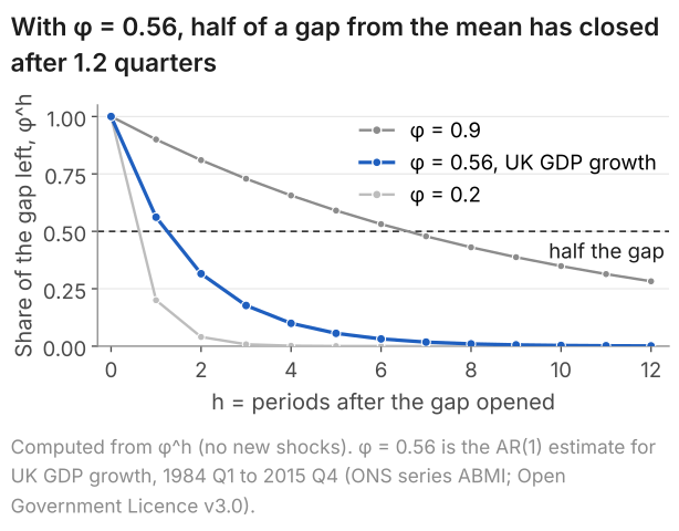
The half-life is the number of periods after which half of a gap is left: for \(0 < \phi < 1\), the \(h\) that solves \(\phi^h = 0.5\). Taking logarithms gives \(h \ln\phi = \ln 0.5\), so
$$ \text{half-life} = \frac{\ln 0.5}{\ln \phi} . $$In words: half-life = the logarithm of one half divided by the logarithm of the coefficient.
Both logarithms are negative; the closer \(\phi\) is to 1, the closer \(\ln\phi\) is to zero and the longer the half-life. For GDP growth it is \(\ln 0.5/\ln 0.5616\), that is \((-0.6931)/(-0.5770) = 1.20\) quarters; for \(\phi = 0.9\), 6.58 periods; for \(\phi = 0.2\), 0.43, so more than half of a gap goes in one period. With \(\phi = 1\), a random walk, \(\phi^h = 1\) and a shock never fades.
4. Estimating it: UK GDP growth, 1984 to 2015
To forecast we need numbers for \(\alpha\), \(\phi\) and \(\sigma\), estimated from the one history we have. The AR(1) is the model; OLS is the method that estimates it, as a regression of growth \(y_t\) on a constant and last quarter's growth \(y_{t-1}\) (lesson 9). The first quarter, 1984 Q1, enters only as a regressor, so 128 quarters give \(n = 127\) pairs, and the residual standard error \(\hat\sigma\), with divisor \(n - 2\) (lesson 10), estimates \(\sigma\).
| Estimate | Std. error | t | 95% interval | |
|---|---|---|---|---|
| Intercept, \(\hat\alpha\) | 0.2462 | 0.0650 | 3.79 | 0.12 to 0.37 |
| Last quarter's growth, \(\hat\phi\) | 0.5616 | 0.0739 | 7.60 | 0.42 to 0.71 |
\(\hat\sigma = 0.5598\) points; \(R^2 = 0.316\). The intervals use the t multiple 1.979, with 125 degrees of freedom (lesson 11). Four decimal places are kept for the hand calculations below.
The code reads uk-gdp-growth.csv: UK GDP for each quarter from 1955 Q1 to 2026 Q2, with columns quarter, gdp (£ million, chained volume measures, seasonally adjusted) and growth (per cent, to four decimals). Save it in your working folder first. The code recomputes growth from gdp at full precision.
R: the code
# AR(1) for UK GDP growth: this quarter's growth on last quarter's, 1984 Q1 to 2015 Q4
gdp <- read.csv("uk-gdp-growth.csv")
# full-precision growth from gdp (the file's growth column has 4 decimals)
gdp$growth <- c(NA, 100 * (gdp$gdp[-1] / head(gdp$gdp, -1) - 1))
d <- subset(gdp, quarter >= "1984Q1" & quarter <= "2015Q4")
d$lag_growth <- c(NA, head(d$growth, -1))  # last quarter's growth (none for 1984 Q1)
fit <- lm(growth ~ lag_growth, data = d)
summary(fit)
confint(fit)
R: what it prints
> # AR(1) for UK GDP growth: this quarter's growth on last quarter's, 1984 Q1 to 2015 Q4
> gdp <- read.csv("uk-gdp-growth.csv")
> # full-precision growth from gdp (the file's growth column has 4 decimals)
> gdp$growth <- c(NA, 100 * (gdp$gdp[-1] / head(gdp$gdp, -1) - 1))
> d <- subset(gdp, quarter >= "1984Q1" & quarter <= "2015Q4")
> d$lag_growth <- c(NA, head(d$growth, -1))  # last quarter's growth (none for 1984 Q1)
> fit <- lm(growth ~ lag_growth, data = d)
> summary(fit)

Call:
lm(formula = growth ~ lag_growth, data = d)

Residuals:
     Min       1Q   Median       3Q      Max
-1.73038 -0.28122  0.00365  0.24271  1.41262

Coefficients:
            Estimate Std. Error t value Pr(>|t|)
(Intercept)  0.24624    0.06500   3.788 0.000235 ***
lag_growth   0.56163    0.07393   7.597 6.19e-12 ***
---
Signif. codes:  0 ‘***’ 0.001 ‘**’ 0.01 ‘*’ 0.05 ‘.’ 0.1 ‘ ’ 1

Residual standard error: 0.5598 on 125 degrees of freedom
  (1 observation deleted due to missingness)
Multiple R-squared:  0.3159,	Adjusted R-squared:  0.3104
F-statistic: 57.72 on 1 and 125 DF,  p-value: 6.189e-12

> confint(fit)
                2.5 %    97.5 %
(Intercept) 0.1175900 0.3748824
lag_growth  0.4153178 0.7079375
Python: the code
import pandas as pd
import statsmodels.formula.api as smf

# AR(1) for UK GDP growth: this quarter's growth on last quarter's, 1984 Q1 to 2015 Q4
gdp = pd.read_csv("uk-gdp-growth.csv")
# full-precision growth from gdp (the file's growth column has 4 decimals)
gdp["growth"] = 100 * gdp["gdp"].pct_change()
d = gdp[gdp["quarter"].between("1984Q1", "2015Q4")].copy()
d["lag_growth"] = d["growth"].shift(1)  # last quarter's growth (none for 1984 Q1)
fit = smf.ols("growth ~ lag_growth", data=d).fit()
print(fit.summary())
Python: what it prints
                            OLS Regression Results
==============================================================================
Dep. Variable:                 growth   R-squared:                       0.316
Model:                            OLS   Adj. R-squared:                  0.310
Method:                 Least Squares   F-statistic:                     57.72
Date:                Sat, 10 Oct 2026   Prob (F-statistic):           6.19e-12
Time:                        21:43:27   Log-Likelihood:                -105.51
No. Observations:                 127   AIC:                             215.0
Df Residuals:                     125   BIC:                             220.7
Df Model:                           1
Covariance Type:            nonrobust
==============================================================================
                 coef    std err          t      P>|t|      [0.025      0.975]
------------------------------------------------------------------------------
Intercept      0.2462      0.065      3.788      0.000       0.118       0.375
lag_growth     0.5616      0.074      7.597      0.000       0.415       0.708
==============================================================================
Omnibus:                       10.929   Durbin-Watson:                   2.068
Prob(Omnibus):                  0.004   Jarque-Bera (JB):               18.098
Skew:                          -0.380   Prob(JB):                     0.000118
Kurtosis:                       4.686   Cond. No.                         2.18
==============================================================================

Notes:
[1] Standard Errors assume that the covariance matrix of the errors is correctly specified.
The row lag_growth holds \(\hat\phi\): in the fitted rule, a quarter one point above the mean is followed, on average, by one 0.56 points above it. The usual t-test is valid in large samples when \(|\phi| < 1\) and the shocks are independent with constant variance (module notes). If \(\phi\) were 0, a t-statistic at least as far from zero as 7.60 would then arise with probability below 0.0005 (lesson 8): strong evidence against \(\phi = 0\). The data are compatible with \(\phi\) from 0.42 to 0.71: half-lives of 0.8 to 2.0 quarters.
From the unrounded estimates the implied mean is 0.5617, or 0.56%, close to the mean of the 128 quarters, 0.57%; the forecasts below use 0.5617. From the estimates rounded to two places, \(0.25/(1 - 0.56)\) would give 0.57 instead.
OLS on a correctly specified AR(1) is consistent but biased downwards in small samples when \(\phi\) is positive, because the regressor is the series' own past. Serial correlation left in the residuals is tested with the Breusch-Godfrey test, not with the Durbin-Watson statistic in the Python printout, 2.068, which is not valid when a lagged dependent variable is a regressor (Durbin-Watson). And the fitted AR(1) is a simple rule, not the process itself: over 1984 to 2019, \(r(2) = 0.416\) exceeds \(r(1)^2 = 0.556^2 = 0.309\) (lesson 23), so an AR(2) or an ARMA(1,1) are other candidates.
5. The forecast one quarter ahead and its error
The first forecast is for the next quarter. We stand at the end of quarter \(T\), here 2015 Q4: \(y_1, \dots, y_T\) are known and \(Y_{T+1}\) is not. Three assumptions carry the derivation.
- The model holds: \(Y_{T+1} = \alpha + \phi Y_T + \varepsilon_{T+1}\).
- The parameters are known. We use the estimates 0.2462 and 0.5616 in their place, and the formulas leave out the error in those estimates.
- Shocks are unpredictable: each has mean zero and is independent of everything before it, a little stronger than white noise, which rules out correlation with the past but not every other link.
Given \(Y_T = y_T\), \(\alpha + \phi y_T\) is a known number (assumptions 1 and 2), and the shock has mean zero whatever happened up to \(T\) (assumption 3). So the expected value of \(Y_{T+1}\) given the data, its conditional mean, is the forecast
$$ \hat Y_{T+1} = \alpha + \phi\,y_T = \mu + \phi\,(y_T - \mu) . $$In words: the forecast = the mean of the process + \(\phi\) times today's gap from the mean.
Among all forecasts computed from the data up to \(T\), this one has the smallest expected squared error, the average of (outcome minus forecast) squared over the values \(Y_{T+1}\) could take given the data. That is what "best" means here, not closest to the outcome every time. We use the result without proving it (module notes).
The forecast error, the outcome minus the forecast, is
$$ Y_{T+1} - \hat Y_{T+1} = \varepsilon_{T+1} . $$In words: the one-step forecast error is the next shock.
So it has mean zero and variance \(\sigma^2\), which is also its expected squared error, the mean squared error. For GDP growth its standard deviation is \(\hat\sigma = 0.56\) points.
For 2016 Q1, from growth of 0.5503% in 2015 Q4, the forecast is \(0.2462 + 0.5616 \times 0.5503 = 0.5552\), or 0.56% (we carry four decimal places and round results to two). Growth was 0.54%: an error of -0.02 points.
6. Two quarters ahead, then h quarters
Beyond one quarter the forecast must deal with values not yet observed. Two quarters ahead, \(Y_{T+2} = \alpha + \phi Y_{T+1} + \varepsilon_{T+2}\), and \(Y_{T+1}\) is unknown at \(T\). Under the same assumptions the expected value of \(Y_{T+2}\) given the data is \(\alpha\) plus \(\phi\) times that of \(Y_{T+1}\), so the unseen value is replaced by its forecast:
$$ \begin{aligned} \hat Y_{T+2} &= \alpha + \phi\,\hat Y_{T+1} \\ &= \mu + \phi^2 (y_T - \mu) . \end{aligned} $$In words: the two-step forecast applies the rule to the one-step forecast.
For 2016 Q2 it is \(0.2462 + 0.5616 \times 0.5552 = 0.5580\), again 0.56%. Software, carrying every digit, gives 0.5553 and 0.5581 for the two quarters; both round to 0.56.
Subtracting the forecast from the model leaves \(\phi\) times next quarter's forecast error, \(\varepsilon_{T+1}\), plus the shock after it:
$$ Y_{T+2} - \hat Y_{T+2} = \varepsilon_{T+2} + \phi\,\varepsilon_{T+1} . $$The two shocks are uncorrelated, so their variances add, with \(\phi\) squared:
$$ \operatorname{Var}(Y_{T+2} - \hat Y_{T+2}) = \sigma^2 (1 + \phi^2) . $$In words: the two-step error variance = the shock variance times one plus the coefficient squared.
For GDP growth the error's standard deviation rises from 0.56 to \(0.5598 \times \sqrt{1 + 0.5616^2}\), that is \(0.5598 \times 1.1469 = 0.64\) points. Repeating the steps \(h\) times gives the forecast at horizon \(h\) and its error variance:
$$ \hat Y_{T+h} = \mu + \phi^h (y_T - \mu) , $$In words: the forecast = the mean + \(\phi^h\) times today's gap from the mean.
$$ \begin{aligned} &\operatorname{Var}(Y_{T+h} - \hat Y_{T+h}) \\ &= \sigma^2 (1 + \phi^2 + \dots + \phi^{2(h-1)}) \\ &= \sigma^2\,\frac{1 - \phi^{2h}}{1 - \phi^2} . \end{aligned} $$In words: the error variance = the shock variance times the sum of the squared weights of the \(h\) shocks still to come.
Show where the forecast and its error variance at any horizon come from
- Write the future value in terms of today's gap. Apply the gap form of section 3 \(h\) times: $$ \begin{aligned} Y_{T+h} - \mu &= \phi^h (Y_T - \mu) \\ &\quad + \varepsilon_{T+h} + \phi\,\varepsilon_{T+h-1} \\ &\quad + \dots + \phi^{h-1}\varepsilon_{T+1} . \end{aligned} $$
- Take the expected value given the data. \(Y_T = y_T\) is known, and by assumption 3 each future shock has mean zero whatever happened up to \(T\). So \(\hat Y_{T+h} = \mu + \phi^h (y_T - \mu)\).
- Take the variance of what remains. The error is the future shocks, \(\varepsilon_{T+h-j}\) with weight \(\phi^j\) for \(j = 0, \dots, h - 1\). They are uncorrelated, each with variance \(\sigma^2\), so the variances add and each weight comes out squared: \(\sigma^2(1 + \phi^2 + \dots + \phi^{2(h-1)})\).
- Sum the series. It is geometric with ratio \(\phi^2\), so the bracket is \((1 - \phi^{2h})/(1 - \phi^2)\). When \(|\phi| < 1\), \(\phi^{2h}\) falls towards zero and the variance approaches \(\sigma^2/(1 - \phi^2)\).
The rules for the variance of a sum are in lesson 3; the module notes give the same steps one and two periods ahead.
A shock arriving \(j\) periods before the target date enters the error with weight \(\phi^j\), so each extra period adds a term and, unless \(\phi = 0\), the variance rises with \(h\); when \(|\phi| < 1\) the added terms shrink and it levels off at \(\sigma^2/(1 - \phi^2)\), the variance of the process. Far ahead, today's value no longer helps: the forecast is the mean, and its error is as variable as the process itself.
The table gives the forecasts made at 2015 Q4. Growth then was 0.011 points below the estimated mean, so the forecasts move only from 0.5553 to 0.5617, all 0.56% to two places, while the error's standard deviation climbs to 0.68 points. The last column applies the rule to a quarter one point above the mean, 1.56%: \(0.5617 + \hat\phi^h\), back towards the mean along the curve of Figure 1. The powers \(\hat\phi^h\) are those of the unrounded estimate, 0.56163; from 0.5616 the third would print as 0.1771.
| h | Quarter | \(\hat\phi^h\) | Forecast (%) | Error sd (points) | From 1.56% (%) |
|---|---|---|---|---|---|
| 1 | 2016 Q1 | 0.5616 | 0.56 | 0.56 | 1.12 |
| 2 | 2016 Q2 | 0.3154 | 0.56 | 0.64 | 0.88 |
| 3 | 2016 Q3 | 0.1772 | 0.56 | 0.67 | 0.74 |
| 4 | 2016 Q4 | 0.0995 | 0.56 | 0.67 | 0.66 |
| 8 | 2017 Q4 | 0.0099 | 0.56 | 0.68 | 0.57 |
| 12 | 2018 Q4 | 0.0010 | 0.56 | 0.68 | 0.56 |
| 16 | 2019 Q4 | 0.0001 | 0.56 | 0.68 | 0.56 |
7. The fan for 2016 to 2019, and what happened
A band needs the shape of the error's distribution, so we add a fourth assumption: normal shocks. The \(h\)-step error, a weighted sum of independent normal shocks, is then normal (lesson 4), with mean zero and standard deviation \(\text{sd}(h)\), the square root of the variance in section 6. A normal distribution has 95% of its probability within 1.96 standard deviations of its centre. Hence, if all four assumptions hold, \(Y_{T+h}\) lies within \(1.96\,\text{sd}(h)\) of its forecast with probability 0.95, and the 95% forecast band is
$$ \hat Y_{T+h} \pm 1.96\,\text{sd}(h) . $$In words: the 95% band = the forecast plus and minus 1.96 error standard deviations.
The promise of 0.95 is made before the outcome is known, so if every assumption holds, about one outcome in twenty should fall outside its band over repeated forecasts. A confidence interval is the reverse: its ends vary from sample to sample around a fixed parameter, while here the band is fixed and the outcome varies. The band also treats the estimates as the parameters, leaving out their error, which would widen it.
For 2016 Q1 the band is \(0.5552 \pm 1.96 \times 0.5598\), that is \(0.5552 \pm 1.0972\), from -0.54% to 1.65%. The half-width reaches 1.32 points at four quarters and 1.33, which is \(1.96 \times 0.6766\), from six quarters on. Figure 2 adds 50% and 80% bands (multiples 0.674 and 1.282).
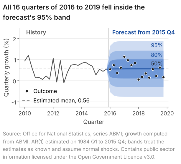
The path is almost flat because 2015 Q4 sat 0.011 points below the estimated mean: with no gap to close, the figure cannot show a return to the mean, which the last column of the table in section 6 shows.
Every outcome fell inside the 95% band, and inside the 80% band too: more than the bands should hold. Under the fitted model the 95% band would miss 0.8 of the 16 quarters on average, and the 50% band would hold about 8; it held 14. The outcomes were less spread out than the model expected. Their standard deviation was 0.32 points, against 0.67 in the estimation sample, and the root mean squared forecast error was 0.31 points, against the 0.67 the model implies. The largest error, 0.58 points in 2017 Q1, was about half the narrowest half-width, 1.10.
The estimation sample includes the recession of 2008 and 2009, with growth of -2.14% in 2008 Q4, and \(\hat\sigma\) was estimated from its shocks; 2016 to 2019 was calmer. So the bands were too wide for these four years, and 16 of 16 inside does not show that they were right. The 16 errors also come from one forecast origin and share shocks, so they are not 16 independent checks.
8. Where forecasts end up
Far ahead, a stationary AR(1)'s forecast is the mean and its error variance levels off; a random walk's does neither. Figure 3 checks the variance formula of section 6 on 10,000 simulated paths for each of \(\phi = 0\), 0.9 and 0.99, with no intercept, standard normal shocks and \(\phi\) known.
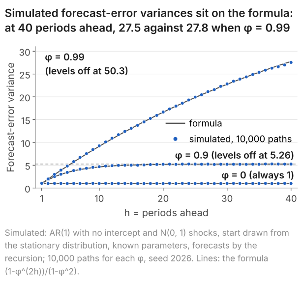
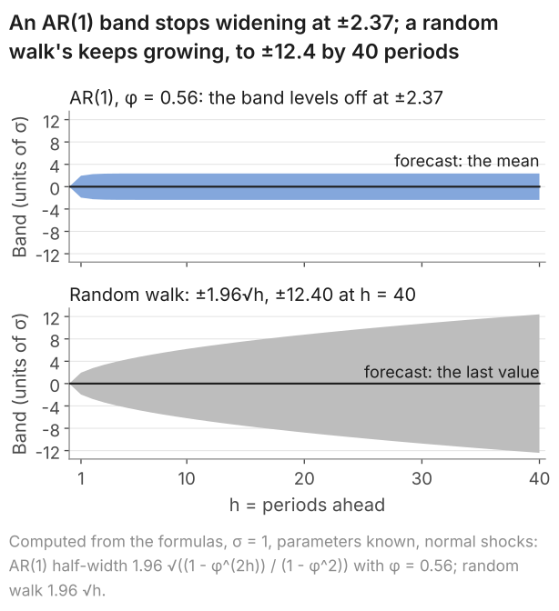
With \(\phi = 0\) the past is no help: the forecast is the mean and the error variance \(\sigma^2\) at every horizon. With \(\phi = 0.9\) the variance is 5.19 by twenty periods, near its limit; with \(\phi = 0.99\) it is 27.76 at forty, 55% of its limit. The more persistent the process, the longer the band keeps widening. GDP growth, with \(\hat\phi = 0.56\), reaches its limit to two places, an error standard deviation of 0.68 points, five quarters ahead.
A random walk, \(\phi = 1\), is never pulled back towards its mean (lesson 24). Its forecast is the last value, and its error after \(h\) periods sums \(h\) shocks at full weight, with variance \(h\sigma^2\), so its band, \(\pm 1.96\,\sigma\sqrt{h}\), keeps widening (Figure 4).
9. The pandemic quarter: what the model could not foresee
The pandemic quarters lie outside both samples and show what a band does not cover. Fitted to 1984 Q1 to 2019 Q4 (143 pairs), the AR(1) gives \(\hat\alpha = 0.2448\), \(\hat\phi = 0.5572\) and \(\hat\sigma = 0.5366\). From growth of -2.83% in 2020 Q1, its forecast for 2020 Q2 is
$$ 0.2448 + 0.5572 \times (-2.8277) = -1.33\% , $$with a 95% band from -2.38% to -0.28%. Growth was -19.93%: an error of -18.60 points, or \(-18.60/0.5366 = -34.7\) residual standard errors, when the largest residual in the 143 quarters fitted was -3.2 residual standard errors (1984 Q2). Fed that fall, the model forecast -10.86% for 2020 Q3; growth was 16.86%, an error of 51.7 residual standard errors. With \(\phi\) positive the rule carries part of every gap forward, so after a fall it forecasts a smaller fall, not a rebound.
The band assumes normal shocks with the variance of 1984 to 2019, and the fall in 2020 Q2 came from the pandemic, not from the series' own past. The pandemic quarters are data, not mistakes; they show that a band speaks only of shocks like those of its sample. We quote no normal tail probability for an error of 35 standard deviations: it would measure how far the normal assumption failed, not how unlikely 2020 was.
10. Common mistakes
- Giving the forecast without its assumptions. When I marked exam answers on AR(1) forecasts, the biggest mistake was not stating the assumptions in the proofs: answers reached the forecasts and the mean squared error without a detailed proof. Name each where it is used: known \(\alpha\) and \(\phi\) and unpredictable shocks for the forecast, uncorrelated shocks with constant variance for the error variance, normal shocks for the band, \(|\phi| < 1\) for the limits.
- Taking the intercept for the mean. For GDP growth \(\hat\alpha = 0.25\) but the mean is 0.56%: \(\mu = \alpha/(1 - \phi)\), computed with three or more decimal places, since \(0.25/(1 - 0.56)\) gives 0.57.
- Applying the rule to the last value at every horizon, or jumping to the mean after one step. From 1.56% the two-step forecast is 0.88%, not 1.12% or 0.56%.
- "The best forecast is the one closest to the outcome." Best means smallest expected squared error. In 2017 Q1 the forecast was 0.56% and growth was 1.14%.
- "The error variance grows without limit." For a stationary AR(1) it levels off at \(\sigma^2/(1 - \phi^2)\), a standard deviation of 0.68 points for GDP growth; a random walk's grows as \(h\sigma^2\).
- "Every outcome fell inside the 95% band, so the model is right." A 95% band should miss about one outcome in twenty; in 2016 to 2019 even the 50% band held 14 of the 16, so the bands were too wide.
- Reading the band as covering the error in the estimates. It treats them as known, though the 95% interval for \(\phi\) runs from 0.42 to 0.71.
11. Check your understanding
Five questions, marked on the page; every option has an explanation, including the wrong ones. (Without JavaScript the explanations are shown beneath each question.)
1. An AR(1) fitted by OLS to UK GDP growth over 1984 Q1 to 2019 Q4 has intercept 0.2448 and coefficient 0.5572. What is the estimated mean of the process, in per cent a quarter?
0.2448/(1 + 0.5572) = 0.16 solves μ = α + φμ with the sign of φμ flipped. Moving φμ to the left gives μ(1 - φ) = α, so μ = 0.2448/0.4428 = 0.55.
0.24 is the intercept. The mean of a stationary AR(1) is α/(1 - φ): each quarter keeps 0.5572 of the level and adds 0.2448, and the level settles at 0.2448/0.4428 = 0.55.
0.2448/(1 - 0.5572²) = 0.2448/0.6895 = 0.36 uses the denominator of the variance, 1 - φ². The mean divides by 1 - φ: 0.2448/0.4428 = 0.55.
Correct. For a stationary AR(1) the mean is μ = α/(1 - φ) = 0.2448/(1 - 0.5572) = 0.2448/0.4428 = 0.55% a quarter, more than twice the intercept.
2. The AR(1) fitted to UK GDP growth over 1984 Q1 to 2019 Q4 has intercept 0.2448, coefficient 0.5572 and an estimated mean of 0.55%. Growth in 2019 Q4 was 0.1606%. What is the forecast of growth in 2020 Q1, in per cent?
0.5572 × 0.1606 = 0.09 leaves out the intercept. The forecast is α + φ y_T = 0.2448 + 0.0895 = 0.33.
0.16 repeats the last value, which would be the forecast of a random walk. With φ = 0.5572 only part of the gap from the mean carries over: 0.2448 + 0.5572 × 0.1606 = 0.33.
Correct. The forecast is 0.2448 + 0.5572 × 0.1606 = 0.2448 + 0.0895 = 0.33: the mean plus 0.5572 times the gap, 0.55 + 0.5572 × (0.16 - 0.55) = 0.33. Growth in 2020 Q1 turned out to be -2.83% as the pandemic began, an error of -5.9 residual standard errors.
0.55 is the mean of the process, the forecast if last quarter carried no information. With φ = 0.5572 it does: the forecast is 0.2448 + 0.5572 × 0.1606 = 0.33.
3. Growth in 2008 Q4 was -2.14%. Applied to that quarter, the AR(1) fitted to 1984 Q1 to 2015 Q4 (intercept 0.2462, coefficient 0.5616, mean 0.56%) gives a forecast for 2009 Q1 of 0.2462 + 0.5616 × (-2.1430) = -0.96%. How is the forecast for 2009 Q2 found?
Correct. Growth in 2009 Q1 is not observed at the end of 2008 Q4, so it is replaced by its forecast: 0.2462 + 0.5616 × (-0.9573) = -0.29%. The gap from the mean shrinks by the factor 0.5616 each quarter, from -2.70 to -1.52 to -0.85 points.
Applying the rule to -2.14 again gives -0.96, the one-step forecast a second time. Two quarters ahead the rule is applied to the value one quarter ahead, which at the end of 2008 is its forecast, -0.96: the result is -0.29%.
The forecast approaches the mean without reaching it: the gap shrinks by the factor 0.5616 each quarter, from -2.70 to -1.52 to -0.85 points. The two-step forecast is 0.2462 + 0.5616 × (-0.9573) = -0.29%.
4. The AR(1) fitted to UK GDP growth over 1984 Q1 to 2015 Q4 has an estimated mean of 0.56%, coefficient 0.5616 and residual standard error 0.5598 points. A forecaster applies it to a quarter of -2.14% growth and looks further and further ahead. What happens to the forecast and to the standard deviation of its error?
That is how a random walk behaves. With φ = 0.5616 the gap from the mean shrinks each quarter, and 0.5616 to the power 16 is 0.0001, so sixteen quarters ahead the forecast is 0.56%; the error's standard deviation stops at 0.68 points.
Correct. The forecast's gap from the mean is 0.5616 to the power h times today's gap of -2.70, which is -0.0003 sixteen quarters ahead, so the forecast becomes the mean. The error variance rises towards σ²/(1 - φ²), whose square root is 0.5598/√(1 - 0.5616²) = 0.68 points, the standard deviation of the process.
The forecast does move to the mean, but the error variance does not grow without limit. Each extra shock enters with a weight 0.5616 to the power j, which shrinks, so the standard deviation levels off: 0.56 points one quarter ahead, 0.64 two ahead and 0.68 from five quarters on.
5. For the AR(1) fitted to UK GDP growth over 1984 Q1 to 2019 Q4, the coefficient is 0.5572 and the residual standard error 0.5366 points, both treated as known. What is the variance of the error of the forecast made two quarters ahead, in squared points?
Correct. The two-step error is the shock two quarters ahead plus φ times the shock one quarter ahead. The shocks are uncorrelated, so the variances add, with φ squared: σ²(1 + φ²) = 0.2879 × 1.3105 = 0.38. Its square root, 0.61 points, is the error's standard deviation.
0.2879/(1 - 0.5572²) = 0.2879/0.6895 = 0.42 is the variance of the process, the limit the error variance approaches far ahead. Two quarters ahead only two shocks are unknown: σ²(1 + φ²) = 0.2879 × 1.3105 = 0.38.
2 × 0.2879 = 0.58 gives both shocks a weight of one. The shock one quarter ahead reaches the quarter after only through the share φ, so its variance is multiplied by φ²: 0.2879 × (1 + 0.3105) = 0.38.
0.2879 × (1 + 0.5572)² = 0.70 adds the weights before squaring. The variance of a sum of uncorrelated terms is the sum of their variances, so each weight is squared on its own: 0.2879 × (1 + 0.3105) = 0.38.
12. Three questions about AR(1) forecasts
An AR(1) model makes each value an intercept plus a share φ of the previous value plus an unpredictable shock. When it is stationary, which needs φ between -1 and 1, its mean is the intercept divided by 1 - φ. For UK GDP growth, 1984 to 2015, φ is estimated at 0.56 and the mean at 0.56% a quarter.
Put the last observed value into the fitted rule: the one-step forecast is the intercept plus φ times that value. For two steps, apply the rule to the one-step forecast, and so on; for a stationary AR(1) the forecasts move back towards the mean. With growth of 0.55% in 2015 Q4, the forecast for 2016 Q1 was 0.56%.
Each extra period adds a shock to the forecast error, so unless φ = 0 its variance rises: σ² one step ahead, σ²(1 + φ²) two steps ahead. For a stationary AR(1) it levels off at the variance of the process; for UK GDP growth the 95% band widens from ±1.10 to ±1.33 points. A random walk's band keeps widening.
13. Where next
- AR, MA and ARMA processes, the explainer: moving-average models, in which today's value depends on a fixed number of past shocks, and the ARMA(1,1), which combines the two kinds of dependence.
- Prediction from an AR(1) in the advanced time series notes, beside the Wold decomposition and the lag operator.
- The module notes on forecast-error variance, with forecasts from an AR(2) and seasonal models.
- Serial correlation and the Breusch-Godfrey test, for checking the residuals of a fitted AR model.
- Lesson 24: stationarity, white noise and random walks (previous), for the condition behind every limit on this page.
- The course home, which lists all 25 lessons and says which are published.
Stuck on a forecasting question? Send it
I tutor econometrics one-to-one, from a first regression through to time series, AR models and forecasting. Bring the question you are stuck on and we will work through it in the free 30-minute consultation.
Book a free 30-minute consultation Econometrics tutor: how it works
Data and simulation. UK GDP: Source: Office for National Statistics, series ABMI; growth computed from ABMI. Contains public sector information licensed under the Open Government Licence v3.0. ABMI is GDP in chained volume measures, seasonally adjusted, £ million, as published on 30 September 2026 and retrieved on 10 October 2026; growth is 100 × (GDP this quarter / GDP last quarter - 1), unrounded. The AR(1) is fitted by OLS to 1984 Q1 to 2015 Q4 (128 quarters, 127 pairs) and, in section 9, to 1984 Q1 to 2019 Q4 (144 quarters, 143 pairs); the forecasts for 2016 Q1 to 2019 Q4 are made at 2015 Q4 with the estimates treated as known. The file the code reads is uk-gdp-growth.csv. Figures 1 and 4 are computed from the formulas. Figure 3 is simulated: for each \(\phi\) in 0, 0.9 and 0.99, a fresh numpy default_rng(2026); first the 10,000 forecast origins, y_T = rng.standard_normal(10000) / sqrt(1 - phi**2), drawn from the stationary distribution; then eps = rng.standard_normal((10000, 40)), row i holding the 40 future shocks of path i; each path follows \(Y_{T+h} = \phi Y_{T+h-1} + \varepsilon_{T+h}\) from \(Y_T = y_T\), the forecasts follow the same recursion without the shocks, and the variance of the errors is taken across the 10,000 paths with divisor R - 1. Adapted from my lecture notes for Time Series Econometrics (ECON30401) at the University of Manchester.