
A scatter of points can be summarised by a straight line, and ordinary least squares (OLS) picks the line whose squared vertical gaps to the points add up to the smallest total. For a small data set that line can be found by hand. We do the arithmetic on five workers, then on 20 Premier League clubs, with three checks.
In this lesson
- Twenty clubs and one line: why a scatter needs a rule
- What the slope formula measures: a picture with four quadrants
- The calculation, step by step, on five workers
- The same arithmetic on 20 real points
- Common mistakes
- Check your understanding: five marked questions
- Three questions about the arithmetic
- Where next
1. Twenty clubs and one line
Here are the 20 Premier League clubs of 2023/24, with goal difference across the page and league points up it. Nobody needs a formula to see the pattern: score more than you concede and you finish higher. The question this lesson answers is narrower. Which straight line summarises the pattern, and how do we find it without a computer?
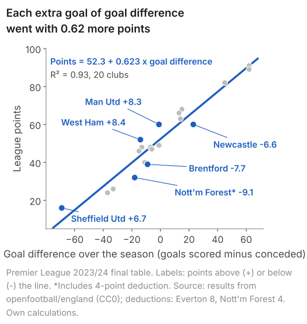
Any line we draw leaves gaps, measured straight up or down from each club's point to the line. The OLS rule is: square every gap, add the 20 squares, and choose the line that makes the total as small as possible. The gaps left by that line are called the residuals. We come back to these clubs in section 4 and compute that line by hand. First we need to see what the formula for the slope measures, and the picture is clearer with five points than with twenty.
Definition: the OLS line
We have \(n\) pairs \((x_i, y_i)\). Take any trial intercept \(b_0\) and trial slope \(b_1\). The line \(b_0 + b_1 x\) misses point \(i\) by \(y_i - b_0 - b_1 x_i\), and the sum of its squared misses is
$$ S(b_0, b_1) = \sum_{i=1}^{n}\bigl(y_i - b_0 - b_1 x_i\bigr)^2 . $$In words: S adds up the squared vertical gaps between the points and the line \(b_0 + b_1 x\).
The ordinary least squares estimates \(\hat\beta_0\) and \(\hat\beta_1\) are the values of \(b_0\) and \(b_1\) at which \(S(b_0, b_1)\) is smallest. The OLS line is \(\hat y = \hat\beta_0 + \hat\beta_1 x\), and the gaps it leaves are its residuals.
Remarks. \(S\) is a function of \(b_0\) and \(b_1\). The \(x_i\) and \(y_i\) are fixed numbers once the sample is collected, so \(S\) changes only when we change the line. For the five workers below, \(S(10, 2) = 2.00\) and \(S(9.6, 2.2) = 1.60\). The Greek letters \(\beta_0\) and \(\beta_1\) stand for the intercept and slope of the true line in the population, which we never see (lesson 10 sets this out). A hat marks the number we compute from the sample to estimate each of them: here, the pair of trial values at which \(S\) is smallest. That pair is unique as long as the x values are not all equal. Other books write \(a\) and \(b\), or \(\alpha\) and \(\beta\); the letters are labels and nothing more.
Least squares: the line with the smallest sum of squared residuals. Ordinary: every point counts equally in that sum. The OLS explainer says why squares and not absolute gaps, with three lines through the same five points.
What students say
“Nicky is an excellent econometrics tutor. He explains complex concepts clearly and makes them much easier to understand.”
“I was completely lost in my economics class, and then I started working Nicky and he totally saved me. He was excellent at explaining the material and extremely accommodating to meet with me many times despite us being in different time zones! Highly recommend working with Nicky!”
“Nicky is a very good and thorough teacher. He has excellent knowledge of econometrics and takes the time to work through your questions. Highly recommended!”
“Really great tutor! Encouraging, knowledgeable, friendly”
“Very good lesson, Nicky is very helpful.”
“Very helpful and clear.”
“I gather it was very useful, thank you!”
“Fantastic!”
2. What the slope formula measures
Five workers, with made-up numbers so that every step fits on one line. \(x\) is years of education after 16 and \(y\) is hourly pay in pounds.
| Worker | x (years) | y (pounds) |
|---|---|---|
| Ana | 0 | 10 |
| Ben | 1 | 12 |
| Cara | 2 | 13 |
| Dev | 3 | 16 |
| Eli | 4 | 19 |
Start with the means: \(\bar x = 10/5 = 2\) and \(\bar y = 70/5 = 14\). Now draw a vertical line at \(x = 2\) and a horizontal line at \(y = 14\). They cross at the point of means, (2, 14), and they cut the picture into four quadrants.
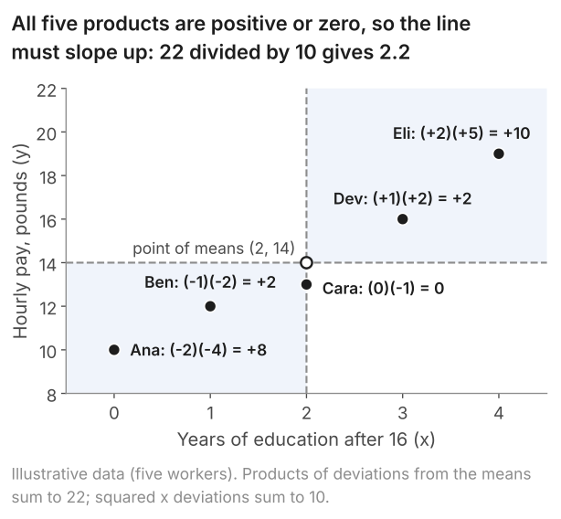
Take Eli. He has two years more education than average and earns £5 more than average, so his two deviations are +2 and +5 and their product is +10. Ana is two years below average and £4 below average: two negative deviations, and their product is +8. In the top-left and bottom-right quadrants one deviation is positive and the other negative, so the product is negative; nobody sits there. Cara sits exactly on the vertical line, so her x deviation is 0 and her product is 0. Add the five products and you get 22.
Intuitively, the total of the products says which way the points lean: up to the right gives a positive total, down to the right a negative one. Points in the top-right and bottom-left quadrants push the total up, points in the other two pull it down, and the balance decides the sign of the slope. That total is the numerator of the slope. Its units are wrong, though: pounds times years, when a slope needs pounds per year. It also grows with the spread of x. Dividing by the sum of the squared x deviations, 4 + 1 + 0 + 1 + 4 = 10 (in years squared), fixes both. Squares are never negative, so the division cannot change the sign. Hence 22/10 = 2.2 pounds an hour per year of education.
$$ \hat\beta_1 = \frac{\sum_{i=1}^{n}(x_i-\bar{x})(y_i-\bar{y})}{\sum_{i=1}^{n}(x_i-\bar{x})^2} $$ $$ \hat\beta_0 = \bar{y} - \hat\beta_1\bar{x} $$In words: slope = sum of the products of deviations, divided by the sum of squared x deviations; intercept = mean of y minus slope times mean of x.
Divide the top and the bottom by \(n\) (or by \(n - 1\)) and you have the sample covariance of x and y over the sample variance of x (lesson 3 defines both). The ratio is the same whichever we divide by, so in computing a slope the division can be left out. The intercept formula says one thing: the line passes through the point of means. Put \(\bar x\) in and you get \(\bar y\) out. The calculus that turns "smallest sum of squares" into these two formulas is set out step by step in the OLS explainer, and in matrix form on the OLS derivation page; we will not need it in this lesson.
3. The calculation, step by step
The same five workers, now as a calculation you can repeat on any small data set. Two passes through the table: one for the means, one for the deviations.
- Means. 2 and 14, from section 2.
- Deviations, products and squares. Subtract 2 from each x and 14 from each y, multiply the pair, and square the x deviation.
The two deviation columns must add to zero. If they do not, a mean is wrong; stop and fix it before going on.
Worker x y x - 2 y - 14 product (x - 2)2 Ana 0 10 -2 -4 8 4 Ben 1 12 -1 -2 2 1 Cara 2 13 0 -1 0 0 Dev 3 16 1 2 2 1 Eli 4 19 2 5 10 4 Sum 10 70 0 0 22 10 - Slope. \(\hat\beta_1 = 22/10 = 2.2\) pounds an hour per year of education.
- Intercept. \(\hat\beta_0 = 14 - 2.2 \times 2 = 9.6\) pounds an hour. The slope comes first; the intercept needs it. Here x = 0 is a real case (a worker who left education at 16), so 9.6 is that worker's fitted pay.
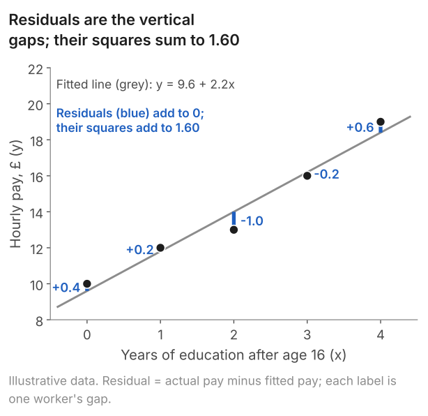
- Fitted values and residuals. Put each x into \(\hat y = 9.6 + 2.2x\) and subtract the fitted value from the actual y.
The squared residuals add to 1.60. This is \(S(9.6,\,2.2)\), the smallest value \(S\) can take for these five workers: the line 10 + 2x, for example, gives \(S(10,\,2) = 2.00\).
Worker y Fitted Residual Residual2 Ana 10 9.6 0.4 0.16 Ben 12 11.8 0.2 0.04 Cara 13 14.0 -1.0 1.00 Dev 16 16.2 -0.2 0.04 Eli 19 18.4 0.6 0.36 Sum 70 70.0 0.0 1.60
If the exam gives you sums instead of a table
A question may give you only \(\sum x\), \(\sum y\), \(\sum xy\) and \(\sum x^2\), and expect the equivalent form:
$$ \sum (x_i-\bar x)(y_i-\bar y) = \sum x_i y_i - n\bar x\bar y $$ $$ \sum (x_i-\bar x)^2 = \sum x_i^2 - n\bar x^2 $$In words: the sum of products of deviations equals the sum of xy minus n times the product of the means; the sum of squared x deviations equals the sum of x squared minus n times the mean of x squared. (Expand the first bracket: \(\sum xy - \bar x \sum y - \bar y \sum x + n\bar x \bar y\), and since \(\sum x = n\bar x\) and \(\sum y = n\bar y\) the last three terms collapse to \(-n\bar x\bar y\).)
For the five workers, the sum of xy is 0(10) + 1(12) + 2(13) + 3(16) + 4(19) = 162 and the sum of x2 is 0 + 1 + 4 + 9 + 16 = 30. So the numerator is 162 - 5 × 2 × 14 = 22 and the denominator is 30 - 5 × 22 = 10: the same two numbers as the table, and the same slope of 2.2. The deviation table is the version to learn from, because it shows what each worker contributes. The sums version is the one to use under time pressure. On one time-series paper I marked, the question supplied a formula as a hint and many scripts re-derived it from scratch instead of using it. If the paper hands you the sums, use them.
4. The same arithmetic on 20 real points
Back to the Premier League. Goal difference is x and points is y. Two facts make this example unusually clean. The mean of goal difference is exactly zero in every season, because every goal scored is a goal conceded by somebody else; so the x deviations are the goal differences themselves. And the mean of points is 1,046/20 = 52.3.
| Club | Goal diff. (x) | Points (y) | y - 52.3 | product | x2 |
|---|---|---|---|---|---|
| Man City | 62 | 91 | 38.7 | 2,399.4 | 3,844 |
| Arsenal | 62 | 89 | 36.7 | 2,275.4 | 3,844 |
| Liverpool | 45 | 82 | 29.7 | 1,336.5 | 2,025 |
| Aston Villa | 15 | 68 | 15.7 | 235.5 | 225 |
| Tottenham | 13 | 66 | 13.7 | 178.1 | 169 |
| Chelsea | 14 | 63 | 10.7 | 149.8 | 196 |
| Newcastle | 23 | 60 | 7.7 | 177.1 | 529 |
| Man United | -1 | 60 | 7.7 | -7.7 | 1 |
| West Ham | -14 | 52 | -0.3 | 4.2 | 196 |
| Crystal Palace | -1 | 49 | -3.3 | 3.3 | 1 |
| Brighton | -7 | 48 | -4.3 | 30.1 | 49 |
| Bournemouth | -13 | 48 | -4.3 | 55.9 | 169 |
| Fulham | -6 | 47 | -5.3 | 31.8 | 36 |
| Wolves | -15 | 46 | -6.3 | 94.5 | 225 |
| Everton | -11 | 40 | -12.3 | 135.3 | 121 |
| Brentford | -9 | 39 | -13.3 | 119.7 | 81 |
| Nott'm Forest | -18 | 32 | -20.3 | 365.4 | 324 |
| Luton | -33 | 26 | -26.3 | 867.9 | 1,089 |
| Burnley | -37 | 24 | -28.3 | 1,047.1 | 1,369 |
| Sheffield Utd | -69 | 16 | -36.3 | 2,504.7 | 4,761 |
| Sum | 0 | 1,046 | 0.0 | 12,004.0 | 19,254 |
Official points, with the season's deductions (Everton 8, Nottingham Forest 4) applied. Because the mean goal difference is 0, the "x - mean" column is x itself and is not repeated.
Slope: 12,004/19,254 = 0.6235 points per goal of goal difference. Intercept: 52.3 - 0.6235 × 0 = 52.3, the average points total. So the line is points = 52.3 + 0.6235 × goal difference.
Software does the same arithmetic. The code below reads the 20 rows from premier-league-2023-24.csv (save it in your working folder first) and fits the line. The two numbers we found by hand, 0.6235 and 52.3, are in the first column of what it prints. The other columns are the subject of lessons 10 and 11.
Stata: the code
import delimited "premier-league-2023-24.csv", clear
regress points gd
Stata: what it prints
. regress points gd

      Source |       SS           df       MS      Number of obs   =        20
-------------+----------------------------------   F(1, 18)        =    233.77
       Model |  7483.95222         1  7483.95222   Prob > F        =    0.0000
    Residual |  576.247782        18  32.0137657   R-squared       =    0.9285
-------------+----------------------------------   Adj R-squared   =    0.9245
       Total |      8060.2        19  424.221053   Root MSE        =    5.6581

------------------------------------------------------------------------------
      points | Coefficient  Std. err.      t    P>|t|     [95% conf. interval]
-------------+----------------------------------------------------------------
          gd |   .6234549   .0407763    15.29   0.000      .537787    .7091227
       _cons |       52.3   1.265183    41.34   0.000     49.64195    54.95805
------------------------------------------------------------------------------
R: the code
# Premier League 2023/24 final table: points (after deductions) and goal difference
pl <- read.csv("premier-league-2023-24.csv")
fit <- lm(points ~ gd, data = pl)
summary(fit)
confint(fit)
R: what it prints
> # Premier League 2023/24 final table: points (after deductions) and goal difference
> pl <- read.csv("premier-league-2023-24.csv")
> fit <- lm(points ~ gd, data = pl)
> summary(fit)

Call:
lm(formula = points ~ gd, data = pl)

Residuals:
   Min     1Q Median     3Q    Max
-9.078 -5.285  0.055  4.253  8.428

Coefficients:
            Estimate Std. Error t value Pr(>|t|)
(Intercept) 52.30000    1.26518   41.34  < 2e-16 ***
gd           0.62345    0.04078   15.29 9.36e-12 ***
---
Signif. codes:  0 ‘***’ 0.001 ‘**’ 0.01 ‘*’ 0.05 ‘.’ 0.1 ‘ ’ 1

Residual standard error: 5.658 on 18 degrees of freedom
Multiple R-squared:  0.9285,	Adjusted R-squared:  0.9245
F-statistic: 233.8 on 1 and 18 DF,  p-value: 9.356e-12

> confint(fit)
                2.5 %     97.5 %
(Intercept) 49.641949 54.9580511
gd           0.537787  0.7091227
Python: the code
import pandas as pd
import statsmodels.formula.api as smf

# Premier League 2023/24 final table: points (after deductions) and goal difference
pl = pd.read_csv("premier-league-2023-24.csv")
fit = smf.ols("points ~ gd", data=pl).fit()
print(fit.summary())
Python: what it prints
                            OLS Regression Results
==============================================================================
Dep. Variable:                 points   R-squared:                       0.929
Model:                            OLS   Adj. R-squared:                  0.925
Method:                 Least Squares   F-statistic:                     233.8
Date:                Thu, 08 Oct 2026   Prob (F-statistic):           9.36e-12
Time:                        14:49:35   Log-Likelihood:                -61.987
No. Observations:                  20   AIC:                             128.0
Df Residuals:                      18   BIC:                             130.0
Df Model:                           1
Covariance Type:            nonrobust
==============================================================================
                 coef    std err          t      P>|t|      [0.025      0.975]
------------------------------------------------------------------------------
Intercept     52.3000      1.265     41.338      0.000      49.642      54.958
gd             0.6235      0.041     15.290      0.000       0.538       0.709
==============================================================================
Omnibus:                        2.895   Durbin-Watson:                   1.352
Prob(Omnibus):                  0.235   Jarque-Bera (JB):                1.209
Skew:                          -0.004   Prob(JB):                        0.546
Kurtosis:                       1.795   Cond. No.                         31.0
==============================================================================

Notes:
[1] Standard Errors assume that the covariance matrix of the errors is correctly specified.
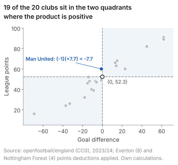
The quadrant picture explains the size of the slope as well as its sign. Sheffield United contribute the largest product, 2,504.7: 69 goals worse than average and 36.3 points below it. Manchester United are the only club in a negative quadrant: a goal difference one below average and 7.7 points above it, product -7.7. The 19 positive products add to 12,011.7 and the one negative product takes 7.7 off, which is why the slope is firmly positive.
Read the slope with its units: each extra goal of goal difference went with 0.62 more points. Aston Villa had a goal difference of +15, so the line predicts 52.3 + 0.6235 × 15 = 61.65 points; they finished on 68, a residual of +6.35. What the line leaves over, the residuals, is the interesting part of this example, and the explainer takes them up.
5. Common mistakes
- Dividing by the wrong sum. The denominator is \(\sum(x_i - \bar x)^2\), the spread of x. Divide by \(\sum(y_i - \bar y)^2\) instead and you get the slope of x on y, a different line that minimises horizontal gaps.
- Forgetting the correction in the sums form. \(\sum xy / \sum x^2\) is not the slope: for the five workers it gives 162/30 = 5.4, not 2.2. Subtract \(n\bar x\bar y\) on top and \(n\bar x^2\) underneath first.
- Rise over run between two points. (19 - 10)/(4 - 0) = 2.25 uses Ana and Eli and ignores the other three. Least squares uses every point, and here it gives 2.2.
- Computing the intercept first. The intercept is \(\bar y - \hat\beta_1 \bar x\), so it needs the slope. Compute the slope first.
- Losing the units. A slope has units. "2.2" does not say what changed; "£2.20 an hour per year of education" does, and so does "0.62 points per goal of goal difference".
- Mixing n and n - 1. Both cancel in the slope. Whichever you divide by, use the same one on top and bottom, or divide by neither, as the tables above do.
6. Check your understanding
Five questions, marked on the page; every option has an explanation, including the wrong ones. (Without JavaScript the explanations are shown beneath each question.)
1. From a sample: the sum of (x - x̄)(y - ȳ) is 30, the sum of (x - x̄)2 is 12 and the sum of (y - ȳ)2 is 90. What is the OLS slope of y on x?
30/90 divides by the spread of y. That is the slope of x on y, a different line. The slope of y on x divides by the spread of x.
12/30 is the formula upside down. The slope is "how y moves per unit of x", so the sum of products goes on top and the x variation underneath.
30/√(12 × 90) = 0.913 is the correlation coefficient. It is unit-free; the slope has units of y per unit of x and equals the correlation times sd(y)/sd(x): 0.913 × 2.74 = 2.5.
Correct. Slope = 30/12 = 2.5: the sum of products of deviations over the sum of squared x deviations.
2. In a scatter of 30 firms, every point lies in the top-left or the bottom-right quadrant around the point of means: above-average x with below-average y, or the reverse. What does this tell you about the OLS slope of y on x?
Top-left and bottom-right both give negative products (one deviation positive, one negative), so they add up rather than cancel. Cancellation happens between a positive quadrant and a negative one.
Correct. A point in either of those quadrants has deviations of opposite sign, so its product is negative. A sum of negative products is negative, and the denominator cannot change the sign. (It is the sum that matters, not the count: one far-out point can outweigh many near the means.)
The denominator is always positive, so it sets the size of the slope and never its sign. The sign comes from the numerator, the sum of the products.
3. In the 2023/24 Premier League regression, points = 52.30 + 0.6235 × goal difference, the intercept 52.30 equals the average points per club exactly. Why?
Correct. Every goal scored is a goal conceded by another club, so the mean of x is zero; intercept = ȳ - slope × x̄ = ȳ.
Only when the mean of x is zero. In general the intercept is ȳ - slope × x̄: for the five workers it is 14 - 2.2 × 2 = 9.6, not 14.
Points are not rescaled or centred; their mean is 52.3. It is goal difference, the x variable, whose mean is zero by construction.
4. Five workers: pay (pounds an hour) on years of education after 16 gives \(\hat y = 9.6 + 2.2x\). How should the 2.2 be read?
A percentage reading needs the log of pay on the left-hand side. In levels the slope is in pounds, and with one regressor nothing else is held fixed.
2.2 is pounds per year, not years per pound. Two workers 2.2 years apart are, on the line, 2.2 × 2.2 = £4.84 apart in pay.
Correct. The slope has units of y per unit of x: pounds an hour per year. "On average" because the line describes the typical worker at each x, and "goes with" because the fit alone does not show that education causes the difference.
5. Why do the residuals from an OLS regression with an intercept always sum to zero?
Errors are unobserved and their sample sum is almost never zero. Residuals are computed from the fitted line, and the fitting is what forces their sum to zero.
Correct. Whatever the slope, the intercept that makes the sum of squares smallest is the one that makes the residuals average zero (with calculus: differentiate with respect to the intercept and set the result to zero). The same step for the slope gives "sum of x times residual = 0", the third check in section 3.
No symmetry is needed. The five-worker residuals are 0.4, 0.2, -1.0, -0.2, 0.6: three above, two below, and they still sum to zero.
7. Three questions about the arithmetic
Neither, unless you want to. The slope is a ratio of two sums, and dividing both by n, or both by n - 1, leaves the ratio unchanged. The choice only matters when you report a covariance or a variance on its own. In a slope calculation, work with the raw sums and divide once.
Compute the two means, then the numerator as the sum of xy minus n times the product of the means, and the denominator as the sum of x squared minus n times the squared mean of x. Divide. For the five workers: (162 - 5 × 2 × 14)/(30 - 5 × 4) = 22/10 = 2.2.
The sum of squared deviations of x, the variable on the right-hand side of the regression. The slope answers "how much does y change per unit of x", so the spread of x goes underneath. Dividing by the spread of y instead gives the slope of x on y, which is a different line.
8. Where next
- Lesson 10: residuals, fit and R-squared, which asks how much of y the line accounts for, using the same five workers and the same 20 clubs.
- What is OLS?, the explainer: why squares rather than absolute values, what the slope and intercept mean, the assumptions in plain words, and six more marked questions.
- The OLS estimator, derived: the calculus behind the formula and the matrix form for several regressors.
- Lesson 8: p-values, Type I and II errors, power (previous) and the course home, which lists all 25 lessons and says which are published.
Send me your regression: module, output and deadline
I tutor econometrics one-to-one, from a first regression through to endogeneity, panel data and time series. Bring the question you are stuck on and we will work through it in the free 30-minute consultation.
Book a free 30-minute consultation Econometrics tutor: how it works
Data and figures. Five-worker example: illustrative data. Premier League: match results from openfootball/england (CC0), 2023/24 season, with the deductions for Everton (8 points) and Nottingham Forest (4 points) applied; sums and products computed for this lesson and checked two ways (the closed-form sums agree with R and statsmodels to better than four significant figures); the 20-row file the code reads is premier-league-2023-24.csv. Figures drawn for this lesson.