
A time series is a variable recorded at successive dates, such as monthly UK inflation. History happened once, so it is unclear in what sense its values are random. Treating the data as one path of a process that could have produced others gives probability statements a meaning, and shows why neighbouring observations need not be a random sample.
In this lesson
- One history: UK inflation since 1989
- The process and the data
- One rule, four histories
- Why a value we have already observed is still treated as random
- Replaying history: inflation 10,000 times
- Positively correlated observations carry less information
- What one history can teach us
- Common mistakes
- Check your understanding: five marked questions
- Three questions about time series
- Where next
1. One history: UK inflation since 1989
The data of this lesson are one real series: the annual rate of UK consumer price inflation in each of the 452 months from January 1989 to August 2026, plotted in Figure 1. Each value is the percentage change in the consumer prices index over the twelve months to that month.
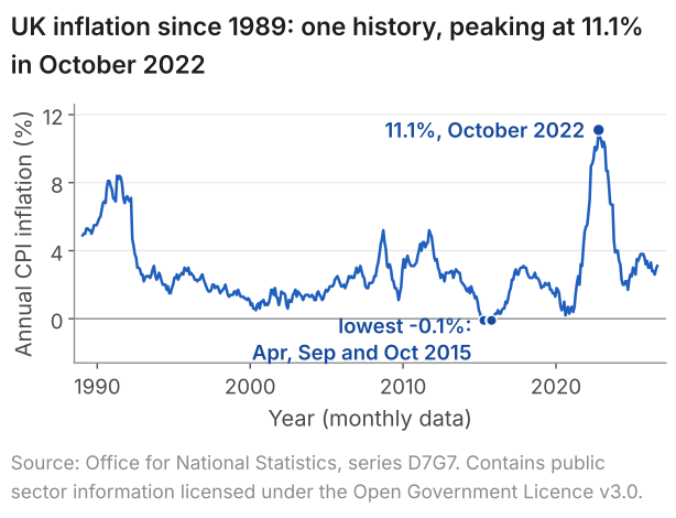
The 60 months above 5% come in five spells: four months in 1989, 31 months from September 1989 to March 1992, one month each in September 2008 and September 2011, and 23 months from November 2021 to September 2023.
The data of lessons 2 to 11 were different. The 1,388 birthweights of lesson 6 were treated as a random sample, each birth drawn independently of the others, so the order of the rows carried no information. A time series differs in two ways.
First, the order is part of the data. Put the 452 months into a random order and the mean and standard deviation do not change, but the spells break up: in one such shuffle the 60 months above 5% fall into 55 separate spells, none longer than three months. In 10,000 shuffles the longest spell above 5% was never more than seven months, against 31 in the actual order.
Second, neighbouring values resemble each other. In 423 of the 451 pairs of neighbouring months, inflation is on the same side of its mean, 2.84%, as in the month before; in the shuffled order, in 240. Part of this is built into the series, since neighbouring annual rates share eleven of their twelve months of price changes. Lesson 22 measures resemblance of this kind in other series.
What students say
“Nicky is an excellent econometrics tutor. He explains complex concepts clearly and makes them much easier to understand.”
“I was completely lost in my economics class, and then I started working Nicky and he totally saved me. He was excellent at explaining the material and extremely accommodating to meet with me many times despite us being in different time zones! Highly recommend working with Nicky!”
“Nicky is a very good and thorough teacher. He has excellent knowledge of econometrics and takes the time to work through your questions. Highly recommended!”
“Really great tutor! Encouraging, knowledgeable, friendly”
“Very good lesson, Nicky is very helpful.”
“Very helpful and clear.”
“I gather it was very useful, thank you!”
“Fantastic!”
2. The process and the data
To say anything about inflation beyond these 452 numbers, we need to separate the mechanism that produces the values from the values it produced.
Definition: process and realisation
A time series process \(Y_t\) is the unknown mechanism that generates the values of a variable at each date \(t\). At each date \(Y_t\) is a random variable: it has a probability distribution over the values it could take. A realisation of the process, also called a sample path, is the set of values the process actually took over the \(T\) dates we observe, written \(y_1, y_2, \dots, y_T\). The realisation is the data, the time series we have.
Remarks. Intuitively, the process is every history that could have occurred, each with its probability, and the realisation is the one that did occur. The process is not the data. The 452 months of Figure 1 are one realisation; the process could have produced others, and we have to learn about it from the one we see.
The notation is that of lesson 2: a capital letter for a random variable, the lower-case letter for the value it takes. Here \(Y_t\) is inflation in month \(t\) as a random variable, and \(y_t\) is the number observed. Counting January 1989 as \(t = 1\), \(y_1 = 4.9\) and, for August 2026, \(y_{452} = 3.1\). \(T\) is the number of periods in the series, here 452. Books use other letters, such as \(X_t\) for the process; the choice is cosmetic.
The sample mean of the 452 months, \(\bar y = 2.84\%\), is a fact about this realisation. If the process has one mean, shared by every month, \(\bar y\) estimates it, and that mean is what a test of a theory about inflation, or a forecast, needs. \(\bar y\) is not that mean, and another realisation could give another value.
In lessons 2 to 11, \(X_1, \dots, X_n\) were \(n\) independent draws from one population, which is random sampling. Here \(Y_1, \dots, Y_T\) may depend on one another and need not share one distribution, and the 452 months are a single draw of a 452-month history, not 452 independent draws.
3. One rule, four histories
A simulation shows what real data never can: several histories from one process. Take the rule
$$ Y_t = 0.1 + 0.4\,Y_{t-1} + \varepsilon_t , $$where each shock \(\varepsilon_t\) is drawn independently from a normal distribution with mean 0 and variance 1.
In words: this period's value = 0.1 + 0.4 times last period's value + a fresh random shock.
The 0.4 carries part of last period's value into this one, which makes neighbouring values resemble each other. The shock is the new, unpredictable part, and the 0.1, together with the 0.4, sets the level around which the values move. In the long run, once the starting value no longer matters, the mean \(\mu\) of the process is the same at every date, so taking expectations of both sides, with shocks of mean 0, gives \(\mu = 0.1 + 0.4\mu\) and \(\mu = 0.1/(1 - 0.4) = 0.167\). Each value then has standard deviation 1.091 (lesson 25 shows where this comes from). A rule of this form is called an autoregression, because the series depends on its own past, and first-order because only the last period enters: AR(1) for short.
We started four paths at \(Y_0 = 0\), gave each its own 100 independent shocks, and applied the rule for \(t = 1\) to 100. The start at 0 holds the early values down: the expected value is 0.1 at \(t = 1\), 0.14 at \(t = 2\) and 0.165 at \(t = 5\).
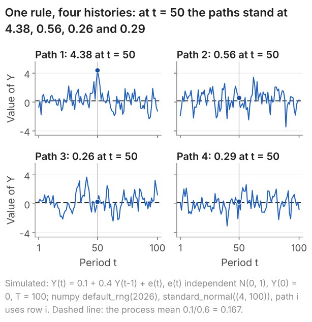
default_rng(2026), standard_normal((4, 100)), path i uses row i.The four paths share the rule and the starting value; only their shocks differ. Yet their means differ from one another and from the process mean, 0.167. At \(t = 50\) path 1 stands at 4.38, its highest value and about 3.9 standard deviations above the process mean, while the other three stand at 0.56, 0.26 and 0.29. Nothing in the rule changed at \(t = 50\): one realisation can stray far from the centre of the process.
Shown only path 4, we would estimate the mean of the process at 0.07; shown only path 2, at 0.34. Across all the paths this rule could produce, the path mean has a standard deviation of 0.166, about half as much again as the 0.109 that 100 independent values with the same spread would give.
The aim of time series analysis is the reverse of this simulation. From the one path we see, such as the 452 months of inflation, we want to infer the form of the process that produced it, and to say how much a statistic computed from that path would vary across the other paths the process could have produced.
4. Why a value we have already observed is still treated as random
The process view treats every observed value as the outcome of a random variable, and at first this may seem odd. Once we know \(y_t\), say UK CPI inflation for September 2016, published as 1.0%, there is no randomness left in it.
However, in August 2016 the rate for the following month was uncertain. Namely, there was some probability that inflation for September 2016 would lie in any given range of values. \(Y_t\) for September 2016 is the random variable that carries those probabilities, and 1.0% is the value it took. The randomness is not doubt about the published figure; it is the variation across the histories the process could have produced.
Hence a probability statement about inflation is a statement about the process, not about the one history we hold. The logic is that of lesson 6, where the 95% belongs to the method of building intervals, across repeated samples, and not to the one interval computed. A forecast with a band around it is a statement of this kind made before the value is known: a range for next month's inflation with a probability attached (lesson 25 builds one).
5. Replaying history: inflation 10,000 times
This section puts numbers on the histories that section 4 appealed to. If we could go back to January 1989 and let the world play out again, we would see a different set of monthly rates, and repeating the experiment would give a set of alternative histories, each with its own probability. Intuitively, the process governs those probabilities. We cannot rerun the UK economy, but we can fit a simple rule to the data and rerun the rule. Everything in this section is a statement about that rule, not about what could have happened to the UK.
The rule has the form of section 3: a constant, plus a fixed share of last month's inflation, plus a shock. We fitted it by OLS (lesson 9), regressing each month's inflation on the month before over the 451 pairs of neighbouring months, February 1989 to August 2026 (lesson 25 covers this step). The fitted rule is
$$ Y_t = 0.0417 + 0.9839\,Y_{t-1} + \varepsilon_t , $$with independent normal shocks whose standard deviation, estimated from the residuals, is 0.368 percentage points.
In words: this month's inflation = 0.0417 + 0.9839 times last month's + a shock with standard deviation 0.368 points.
The coefficient 0.9839 makes the rule highly persistent. Its long-run mean is \(0.0417/(1 - 0.9839) = 2.59\%\), and on average a gap from that mean halves in about 43 months (lesson 25 shows the calculation). The series ends 1.8 points below where it starts, and for an AR(1) fitted by OLS the rule's mean differs from the sample mean by about that change divided by the 451 pairs and by \(1 - 0.9839\): \(-1.8/(451 \times 0.0161) = -0.25\) points, which puts it below the sample mean of 2.84%.
A replay starts the rule where inflation started, at 4.9% in January 1989, draws 451 independent shocks with standard deviation 0.368, and applies the rule month by month to August 2026. Figure 3 sets 20 replays beside the actual series.
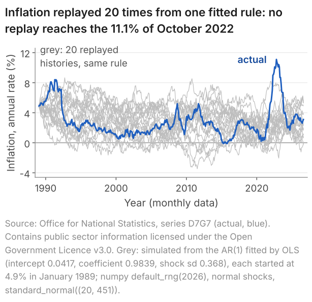
default_rng(2026), standard_normal((20, 451)) times the fitted 0.368.Each grey line is a history the rule could have produced; the blue line is the one that occurred. Over 10,000 replays, the share in which something happens is its probability under the rule, up to simulation error. For example, 5,289 of the 10,000 replays end between 1% and 4% in August 2026, so under the rule, starting from 4.9% in January 1989, that outcome has a probability of about 53%.
In some respects the actual history looks like a typical replay. The median replay spends 57 months above 5%, against 60 in the actual history, and 48.3% of replays spend at least 60. Across the 10,000 replays the median August 2026 value is 2.6%, and 90% of the August 2026 values lie between -0.8% and 6.0%; the actual 3.1% is well inside that range.
In two respects it does not. The first is the peak: none of the 20 replays reaches 11.1%, and only 24 of the 10,000 do, 0.24%; in 95% of replays the highest value reached is below 9.1%. The second is the floor: 8,091 of the 10,000 replays go below zero at some point, and the median replay spends 21 months below zero. The actual series spent 3 months below zero and never went lower than -0.1%.
The replays come from a simple rule fitted to the data, not from the process that produced UK inflation. So these disagreements are evidence about the rule; they do not show that the inflation of 2022 had a probability of 0.24%. A rule whose shocks all have one size has one spread: in the long run its standard deviation is 2.06 points. That is about twice the 0.99 points of the calm years from January 1993 to December 2019, and two-thirds of the 3.11 points since January 2020 (lesson 22 shows this kind of change). So the replays wander below zero far more than the actual series did, and rarely reach the surge of 2022. The rule is a rough stand-in for an unknown process, and the comparison shows where it falls short.
6. Positively correlated observations carry less information
Dependence between neighbours changes how much a series of a given length can teach us, and the sample mean is the simplest place to see it. What we are after is how far the mean of \(T\) observations, \(\bar Y\), lies from the mean of the process, across the paths the process could produce. As in lessons 4 and 5, the measure is the variance of the sample mean: the average squared distance between \(\bar Y\) and the mean of the process, over all those paths.
Write \(\sigma_Y^2\) for the variance of one observation (the subscript keeps it apart from the variance of the shocks; lesson 23 writes it \(\gamma(0)\)). The variance of a sum is the sum of the variances plus twice the covariance of every pair (lesson 3). If the \(T\) observations are independent, every covariance is zero, so the variance of their mean is \(\sigma_Y^2/T\) (lesson 4); its square root, \(\sigma_Y/\sqrt{T}\), is what the standard error \(s/\sqrt{T}\) estimates (lesson 5).
In a time series the covariances need not be zero. When neighbouring values are positively correlated, each such covariance adds to the variance of the sum, so the sample mean varies more from path to path than \(\sigma_Y^2/T\) says. In essence, the high and low values that offset one another in a mean of independent observations arrive in runs, and a run moves the mean as a block.
Suppose every observation has variance \(\sigma_Y^2\), and the correlation between two observations depends only on how far apart they are: \(\rho(k)\) for two observations \(k\) periods apart (the autocorrelation of lesson 23). Then
$$ \operatorname{Var}(\bar Y) = \frac{\sigma_Y^2}{T} \times B , $$ $$ B = 1 + 2\sum_{k=1}^{T-1}\Big(1 - \frac{k}{T}\Big)\rho(k) . $$In words: variance of the mean of dependent observations = the formula for independent observations times a factor \(B\) that adds up the correlations between all pairs.
Show where the variance of the mean comes from
- Write the mean as a sum. \(\bar Y = \frac{1}{T}(Y_1 + \dots + Y_T)\). A constant comes out of a variance squared, so $$ \begin{aligned} &\operatorname{Var}(\bar Y) \\ &= \frac{1}{T^2}\operatorname{Var}(Y_1 + \dots + Y_T) . \end{aligned} $$
- Use the variance of a sum. It is the sum of the \(T\) variances plus twice the covariance of every pair. The variances add to \(T\sigma_Y^2\). If every covariance were zero, dividing by \(T^2\) would give \(\sigma_Y^2/T\), the formula of lessons 4 and 5.
- Group the pairs by distance. Two observations \(k\) periods apart have covariance \(\rho(k)\,\sigma_Y^2\): their correlation times the product of their standard deviations (lesson 3). There are \(T - k\) such pairs, from \((Y_1, Y_{1+k})\) to \((Y_{T-k}, Y_T)\), so the pairs \(k\) apart contribute \(2(T - k)\,\rho(k)\,\sigma_Y^2\).
- Divide by \(T^2\). Taking \(\sigma_Y^2/T\) outside, the variances give 1 and the pairs \(k\) apart give \(2(1 - k/T)\,\rho(k)\), since \((T - k)/T = 1 - k/T\). Adding these over \(k = 1\) to \(T - 1\) gives \(B\), so \(\operatorname{Var}(\bar Y) = (\sigma_Y^2/T) \times B\).
For the rule of the table below, \(\rho(k) = \phi^k\) (lesson 25). With \(T = 100\) the sum gives \(B = 2.311\) at \(\phi = 0.4\) and \(B = 17.20\) at \(\phi = 0.9\), so \(0.1091 \times \sqrt{2.311} = 0.166\) and \(0.2294 \times \sqrt{17.20} = 0.951\), as in the table. As \(T\) grows, \(B\) approaches \((1 + \phi)/(1 - \phi)\): 2.333 at \(\phi = 0.4\) and 19 at \(\phi = 0.9\). So in a long series \(T\) observations are worth about \(T(1 - \phi)/(1 + \phi)\) independent ones: 42.9 and 5.3 for \(T = 100\), a little below the exact 43.3 and 5.8.
For independent observations every \(\rho(k)\) is zero and \(B = 1\), which is lessons 4 and 5 again. Each correlation enters twice, once for each order of the pair, with the weight \(1 - k/T\), because only \(T - k\) pairs of observations are \(k\) periods apart. \(B\) is a pure number; the variance of the mean is in the squared units of the series, and its square root, the standard deviation of the mean, in the units of the series.
The table sets the formula beside a simulation of \(Y_t = \phi\,Y_{t-1} + \varepsilon_t\), with independent N(0, 1) shocks, for \(\phi = 0\) (independent observations), 0.4 (the dependence of section 3's rule) and 0.9. Each path has \(T = 100\) observations and starts from a random draw from the distribution the rule settles into in the long run, so every observation has the same variance and the assumptions of the formula hold. For each \(\phi\) we drew 10,000 paths and computed each path's mean.
| \(\phi\) | Std. deviation of one observation, \(\sigma_Y\) | Std. deviation of the mean if independent, \(\sigma_Y/\sqrt{100}\) | Exact std. deviation of the mean | In these 10,000 paths | Equivalent number of independent observations, \(T/B\) |
|---|---|---|---|---|---|
| 0 | 1.000 | 0.100 | 0.100 | 0.099 | 100 |
| 0.4 | 1.091 | 0.109 | 0.166 | 0.163 | 43.3 |
| 0.9 | 2.294 | 0.229 | 0.951 | 0.936 | 5.8 |
At \(\phi = 0\) the independent-data formula and the exact standard deviation of the mean agree, as lessons 4 and 5 say they must. At \(\phi = 0.4\) the mean of 100 observations varies with a standard deviation of 0.166, not 0.109: 1.52 times as much. At \(\phi = 0.9\) it is 0.951, not 0.229: 4.15 times as much. The simulated column agrees with the exact one up to simulation error. In this run each simulated figure is a little below the exact one, by about two of its standard errors, and the three rows share the same random draws, so the three shortfalls are not independent.
The last column turns this into a count. A mean of independent observations has variance \(\sigma_Y^2\) divided by their number, so the number of independent observations whose mean is as precise as ours is \(T/B\). At \(\phi = 0.4\), \(100/2.311 = 43.3\): the 100 dependent observations pin down the mean of the process as well as 43 independent ones would. At \(\phi = 0.9\), \(100/17.20 = 5.8\): as well as about 6.
So the standard error of lesson 5, \(s/\sqrt{T}\), is the wrong measure of precision for the mean of dependent observations. It estimates \(\sigma_Y/\sqrt{T}\), the third column, and at \(\phi = 0.9\) that is less than a quarter of the 0.951 it should be (0.229/0.951 = 0.24). Real data can show dependence at least this strong: the rule fitted to inflation in section 5 carries 0.98 of each month's value into the next. Lesson 23 measures dependence of this kind from the data.
7. What one history can teach us
Everything we learn about a process comes from the one path we observe, and two conditions decide how much that path can teach.
- The process must be stable over the sample. If the mean or the variance of \(Y_t\) changed from month to month, each month would be the only draw from its own distribution, and 452 months would say little about any one of them; the condition that rules this out, stationarity, is the subject of lesson 24.
- The sample must be long enough. With three quarterly observations it is difficult to tell one process from another, and section 6 showed that positive dependence makes a series worth fewer independent observations than its length; lesson 23 shows how much data a measure of dependence needs.
8. Common mistakes
- "The mean of the series is the mean of the process." The mean of the 452 months, 2.84%, estimates the mean of the process. Four paths of one rule whose mean is 0.167 have means from 0.07 to 0.34.
- "A value that has been observed cannot be random." In August 2016 inflation for September was uncertain; the published 1.0% is the value that random variable took.
- "The replays show what could have happened to UK inflation." They show what the fitted rule produces: that 24 of 10,000 reach 11.1% says the rule describes 2021 to 2023 poorly, not that 2022 had a probability of 0.24%.
- Treating \(T\) observations of a time series as a random sample of size \(T\). The standard error \(s/\sqrt{T}\) assumes independent observations. With \(\phi = 0.9\) the mean of 100 observations varies with a standard deviation of 0.951, not 0.229.
- "Shuffling the months loses nothing, since the mean and standard deviation are unchanged." A shuffle destroys the order: in one shuffle the 60 months above 5% fall into 55 spells instead of five.
9. Check your understanding
Five questions, marked on the page; every option has an explanation, including the wrong ones. (Without JavaScript the explanations are shown beneath each question.)
1. UK CPI inflation averaged 2.84% over the 452 months from January 1989 to August 2026. Which statement about this 2.84% is right?
The 452 months are one realisation of the process, and 2.84% is computed from them. It estimates the mean of the process but is not that mean: in the lesson's simulation, four paths of one rule whose mean is 0.167 have means of 0.25, 0.34, 0.32 and 0.07.
Correct. 2.84% is the value the sample mean took in the one history we have, and it estimates the mean of the process. The process could have produced other histories, each with its own mean, as four paths of one simulated rule have means from 0.07 to 0.34 around a process mean of 0.167.
2.84% is fixed now, but it is one outcome of the process, which is why it can estimate the mean of the process at all. What remains is to measure how far such means vary from one history to another, which is what section 6 does.
2. Figure 2 shows four paths of 100 periods from the rule \(Y_t = 0.1 + 0.4\,Y_{t-1} + \varepsilon_t\), each started at \(Y_0 = 0\). At \(t = 50\) they stand at 4.38, 0.56, 0.26 and 0.29. What makes the four paths differ?
All four paths use the same rule, with the same two numbers, and the same start. Paths from one rule differ because their shocks differ: path 4's mean, 0.07, and path 2's, 0.34, come from the same 0.1 and 0.4.
4.38 is about 3.9 standard deviations of the process (1.091) above its mean, 0.167, yet it comes from the same rule as the other three paths. One realisation can stray far from the centre of the process without any change in the rule.
Correct. The rule and the starting value are the same for all four, and each path uses its own row of 100 independent N(0, 1) shocks. The shocks alone produce values at t = 50 from 0.26 to 4.38 and path means from 0.07 to 0.34.
3. The process \(Y_t = 0.9\,Y_{t-1} + \varepsilon_t\), with independent N(0, 1) shocks, has settled into its long-run distribution, in which each observation has standard deviation 2.294. For 100 consecutive observations, the factor \(B\) by which this dependence multiplies the variance of their mean is 17.20. Across all possible paths, what is the standard deviation of the mean of the 100 observations?
2.294/100 = 0.023 divides by the number of observations. Even for independent observations the divisor is √100 = 10, and dependence makes the figure larger still: the lesson's table gives 0.951.
1/√100 = 0.1 uses the standard deviation of the shocks, 1, in place of that of an observation, 2.294, and also treats the observations as independent. With φ = 0.9 the mean of 100 observations has standard deviation 0.951.
2.294/√100 = 0.229 is the formula of lessons 4 and 5, which assumes independent observations. Here neighbouring values are strongly positively correlated, so every covariance adds to the variance of the sum: the exact figure is 0.951, 4.15 times 0.229.
Correct. The variance of the mean is the independent-data value, 2.294²/100, times B = 17.20, so its standard deviation is 0.2294 × √17.20 = 0.951: more than four times the 0.229 of the independent-data formula, because the positive correlations add to the variance of the sum. In the lesson's 10,000 simulated paths it was 0.936.
4. Lesson 21 replays UK inflation 10,000 times from an AR(1) fitted by OLS to the 452 months, each replay starting at 4.9% in January 1989. 24 of the 10,000 replays reach 11.1%, the peak of October 2022. What does this number show?
Correct. The share of replays with a property estimates its probability under the rule that produced them: 24 of 10,000 is 0.24%, with a simulation standard error of about 0.05 percentage points. It is a statement about the rule, an AR(1) with shocks of one size, not about how likely 2022 was.
The replays come from the fitted rule, not from the UK economy, so 0.24% is a probability under that rule. The actual series did reach 11.1%, which is evidence that the rule describes 2021 to 2023 poorly, not that 2022 had a 0.24% chance.
With 10,000 replays a share of 0.24% has a simulation standard error of about 0.05 percentage points, so it is estimated well enough to compare with the data. More replays would narrow the estimate of 0.24%, not overturn it.
5. The 452 monthly inflation rates of Figure 1 are put into a random order. Which feature of the data does that change?
A mean and a standard deviation use each value once, whatever the order, so a shuffle leaves them at 2.84% and 2.13 points. What a shuffle changes is which values sit next to each other.
For a random sample, such as lesson 6's births, the order of the rows carries no information. In a time series it does: in the actual order 423 of the 451 neighbouring pairs are on the same side of the mean, and the 60 months above 5% come in five spells.
Correct. A shuffle keeps every value but breaks the link between neighbours. In one shuffle the 60 months above 5% fall into 55 spells, none longer than three months, against five spells and a longest of 31 months in the actual order; the 423 of 451 neighbouring pairs on the same side of the mean become 240.
10. Three questions about time series
A time series is one variable recorded at successive dates, such as UK CPI inflation in each of the 452 months from January 1989 to August 2026. Its order matters and neighbouring values resemble each other: in 423 of the 451 pairs of neighbouring months, inflation is on the same side of its mean as in the month before.
The process is the unknown rule that gives each date a probability distribution of possible values; a realisation is the one set of values it produced, the data. One rule can produce any number of realisations: four simulated paths of the same rule have means of 0.25, 0.34, 0.32 and 0.07, around a process mean of 0.167.
Cross-sectional data, such as 1,388 birthweights, are treated as independent draws, so their order carries no information. A time series is one path of a process: its order matters, and neighbouring observations may be dependent. Positive dependence costs information: the mean of 100 observations of an AR(1) with coefficient 0.9 is as precise as that of about 6 independent ones.
11. Where next
- Lesson 22: reading a time-series graph, which names the features to look for in a plot of a series and attaches a number to each.
- Time series econometrics notes, the explainer that sets out the first definitions of time series on one page, with this lesson's idea in brief.
- The lecture notes on processes, stationarity and white noise, for the same ideas with the algebra.
- The lecture note on estimating the mean of a time series, for the other half of section 6: if the process is stationary and the dependence between distant dates dies away, the sample mean still settles on the mean of the process as the series lengthens, more slowly when the positive dependence is strong.
- The course home, which lists all 25 lessons and says which are published.
Stuck on a time series question? Send it
I tutor statistics and econometrics one-to-one, from a first time series plot through to ARMA models, forecasting and panel data. Bring the question you are stuck on and we will work through it in the free 30-minute consultation.
Book a free 30-minute consultation Econometrics tutor: how it works
Data and simulation. Inflation: Source: Office for National Statistics, series D7G7 (CPI annual rate, all items, monthly, January 1989 to August 2026, 452 months; release of 16 September 2026, retrieved 10 October 2026). Contains public sector information licensed under the Open Government Licence v3.0. Shuffles (section 1): a fresh numpy default_rng(2026) and its permutation(452) for the one shuffle described, and 10,000 permutations drawn in turn from one fresh default_rng(2026), the first being that shuffle. Four paths (Figure 2): \(Y_t = 0.1 + 0.4\,Y_{t-1} + \varepsilon_t\), shocks independent N(0, 1), \(Y_0 = 0\), \(T = 100\); a fresh default_rng(2026) and standard_normal((4, 100)), path i uses row i. Replays (Figure 3 and section 5): the AR(1) fitted by OLS to the 452 months (451 pairs; intercept 0.0417, coefficient 0.9839, residual standard deviation 0.368, divisor 449; the replays use the unrounded estimates), each replay started at 4.9% in January 1989 and run to August 2026 with normal shocks of the fitted standard deviation; a fresh default_rng(2026) and standard_normal((20, 451)) for the 20 of the figure, and a second fresh generator and standard_normal((10000, 451)) for the 10,000, whose first 20 rows are the figure's. Table of section 6: \(Y_t = \phi\,Y_{t-1} + \varepsilon_t\), shocks independent N(0, 1), \(Y_1\) drawn from N(0, 1/(1 - \(\phi^2\))), \(T = 100\), 10,000 paths for each \(\phi\); a fresh default_rng(2026) for each \(\phi\) and standard_normal((10000, 100)), so the three rows use the same draws. Adapted from my lecture notes for Time Series Econometrics (ECON30401) at the University of Manchester.