
To model a series we need to know how it behaves: whether it trends, repeats each year, stays on one side of its mean, changes its spread or jumps. A time-series graph, the series plotted against time, shows this first. This lesson names six features, puts a number on each and shows what a graph cannot settle.
In this lesson
- A first look: UK GDP since 1955
- Trend, and why we study growth
- Seasonality: retail sales every December
- Persistence and the sign of dependence
- Volatility: IBM's returns, decade by decade
- Outliers and shifts in the mean
- What a graph cannot settle
- Describing a graph in an exam or a report
- Common mistakes
- Check your understanding: five marked questions
- Three questions about time-series graphs
- Where next
1. A first look: UK GDP since 1955
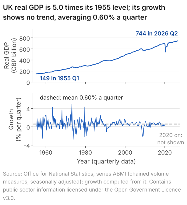
The first step with any time series, a variable recorded at successive dates (lesson 21), is to plot it against time and say what the picture shows, before computing anything. Figure 1 plots UK real GDP, the output of the economy with changes in prices removed, in two forms. The top panel shows its level, which climbs over 71 years with short dips, the deepest in 2020. The bottom panel shows growth, the change from one quarter to the next as a percentage of the level. Growth moves around a flat dashed line with no drift, and its swings are wider before the mid-1980s than after. The panel stops at the end of 2019, for a reason section 6 gives.
What students say
“Nicky is an excellent econometrics tutor. He explains complex concepts clearly and makes them much easier to understand.”
“I was completely lost in my economics class, and then I started working Nicky and he totally saved me. He was excellent at explaining the material and extremely accommodating to meet with me many times despite us being in different time zones! Highly recommend working with Nicky!”
“Nicky is a very good and thorough teacher. He has excellent knowledge of econometrics and takes the time to work through your questions. Highly recommended!”
“Really great tutor! Encouraging, knowledgeable, friendly”
“Very good lesson, Nicky is very helpful.”
“Very helpful and clear.”
“I gather it was very useful, thank you!”
“Fantastic!”
2. Trend, and why we study growth
A trend is a persistent change in the level of a series. Here we measure the trend in GDP and see why the later lessons work with its growth rate instead.
A series with a trend has no single level to describe: the mean of real GDP is £171.5 billion over 1955 to 1964 and £682.6 billion over 2015 to 2024. Growth has no such drift: over 1955 Q2 to 2019 Q4 it moves around a mean of 0.60% a quarter, with a standard deviation of 0.97, and one mean can describe its level. Lesson 24 makes precise what that requires, under the name stationarity.
To compare quarters 71 years apart we need the change in GDP as a share of its size, not in pounds: on the constant prices of the series, £1 billion was 0.67% of GDP in 1955 Q1 but 0.13% in 2026 Q2. So growth in quarter \(t\), written \(g_t\), is the change from the quarter before divided by the level in the quarter before, in per cent:
$$ g_t = 100 \times \left( \frac{\text{GDP}_t}{\text{GDP}_{t-1}} - 1 \right) . $$In words: growth (% a quarter) = 100 × (this quarter's GDP ÷ last quarter's GDP, minus 1).
The ratio puts the two quarters on the scale of the economy at the time; subtracting 1 leaves the change; multiplying by 100 makes it a percentage. With £744.453 billion in 2026 Q2 against £740.509 billion in 2026 Q1 (as published in September 2026), growth is \(100 \times (744.453/740.509 - 1) = 0.53\)% a quarter. As a definition the formula needs no assumption, but GDP must be measured at constant prices, as here, for \(g_t\) to measure growth in output and not a rise in prices. A difference between two rates, such as two growth rates or two unemployment rates, is in percentage points. Lesson 24 shows what taking differences does to a trending series.
From lesson 23 on, the GDP growth examples use the main sample, the 144 quarters from 1984 Q1 to 2019 Q4 (mean 0.56%, standard deviation 0.64), or a stated part of it. We write \(T\) for the number of periods in a series, so here \(T = 144\). Section 6 explains why the quarters from 2020 are left out.
3. Seasonality: retail sales every December
Seasonality is a pattern that repeats each year. We measure it in a series published without seasonal adjustment, the value of UK retail sales (Figure 2).
The top panel mixes two features: a trend, as the yearly mean of the index rises from 39.1 in 1996 to 102.0 in 2025, and a spike every December. To separate them, we divide each month's value by the mean of its own year's twelve months and average this ratio over the 30 complete years, 1996 to 2025. The ratio removes the rise in level from one year to the next and, unlike an excess in index points, does not grow with the level: the same seasonal pattern adds more points when the level is higher. December's average ratio is 1.258, so December is 25.8% above the mean of its year.
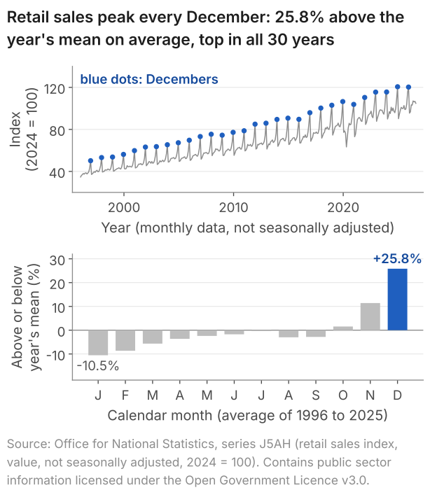
December is the highest month in all 30 years, and January the lowest in 28 of them. The pattern can drift, though: December's ratio averaged 1.281 in 1996 to 2005 and 1.231 in 2016 to 2025, so a pattern measured in one decade need not hold in the next.
Whether a series is seasonally adjusted decides what its graph can show. The Office for National Statistics (ONS) publishes this index unadjusted, so the spike stays in. It publishes GDP and the unemployment rate seasonally adjusted: it estimates the pattern that repeats each year and removes it, so that neighbouring quarters or months can be compared. CPI inflation compares each month's prices with the same month a year earlier, which removes a fixed seasonal pattern by construction. The advanced notes cover models of seasonality, and the module notes cover seasonal adjustment.
4. Persistence and the sign of dependence
Persistence is positive dependence of each value of a series on the one before. We measure it first by counting, on UK unemployment, then build four series that show the sign and size of the dependence.
Figure 3 shows the unemployment rate, seasonally adjusted; each of its 665 values is the rate over three months. It moves in long swings around its mean of 6.61%, and stays above it for 207 consecutive values, from the three months to August 1980 to the three months to October 1997.
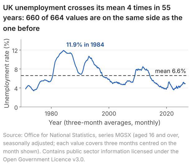
To put a number on this, pair each value with the one before it and count the pairs in which both lie on the same side of the mean: 660 of 664, 99.4%. Suppose instead that the values were independent, with a distribution symmetric about the mean. Then each value would lie above or below the mean with probability one half, whatever the value before, and about half the pairs, some 332, would lie on the same side. 660 is far from 332: unless the mean itself shifts, this is strong evidence that each value depends on the one before, and that the dependence is positive.
Definition: persistence
A process is persistent when the correlation between its value in one period and its value in the next is positive; lesson 23 names this correlation the autocorrelation at lag 1. In a graph, strong positive dependence shows as long spells on one side of the mean, and strong negative dependence as a zigzag across it.
Remarks. Intuitively, a persistent process has memory: its value today depends on its past values. Persistence is not a trend. A trend is a change in the level; persistence is the positive dependence of each value on the one before. Unemployment has the second without the first: it starts at 3.8% and ends at 4.9%, yet it has the highest share in the table below.
The same count compares four series.
| Series | Pairs on the same side of the mean as the one before | Share |
|---|---|---|
| Unemployment rate, as in Figure 3 | 660 of 664 | 99.4% |
| CPI inflation, January 1989 to August 2026 | 423 of 451 | 93.8% |
| GDP growth, 1984 Q1 to 2019 Q4 | 98 of 143 | 68.5% |
| IBM monthly returns, January 1926 to December 2003 | 472 of 935 | 50.5% |
A trend or a shift in the mean also keeps a series on one side of its overall mean for long spells, as section 6 shows for inflation. Some persistence is also built in by how a series is made: neighbouring unemployment values share two of their three months, and neighbouring inflation rates, each comparing a month with a year earlier, share eleven of their twelve months of price changes. GDP growth has no such overlap, so the cleaner comparison is GDP growth, 68.5%, against IBM's returns, 50.5%, about what independent values would give. The correlation between one period's value and the next agrees: 0.56 for GDP growth in the main sample, 0.035 for IBM. Lesson 23 gives its formula; here it matches the ordinary correlation of the pairs to two decimals.
To see what the sign and size of the dependence look like, we build series whose dependence we set ourselves, with the rule
$$ Y_t = \phi\, Y_{t-1} + \varepsilon_t , $$where \(Y_t\) is the value of the process in period \(t\), \(\varepsilon_t\) is a new random shock and \(\phi\) (the Greek letter phi) is a fixed number. We assume the shocks are independent draws from a normal distribution with mean 0 and variance 1, and start each path at \(Y_0 = 0\).
In words: this period's value = \(\phi\) × last period's value + a new shock.
\(\phi\) is the share of last period's value carried into this one. At \(\phi = 0.9\), nine tenths carries over, so a run of positive shocks builds a long spell above zero. At \(\phi = -0.9\) the part carried over changes sign, which pushes the path across zero almost every period. At \(\phi = 0\) the path would be the shocks themselves. The rule has the form of the one in lesson 21, without the intercept, so the paths move around zero; lesson 25 studies it as the AR(1) model. Books use other letters for \(\phi\) and the shocks, and the choice is cosmetic.
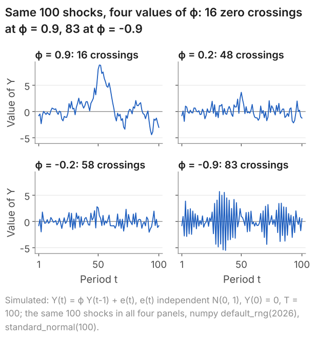
Positive dependence gives long spells and 16 crossings; negative dependence gives a zigzag and 83. Independent values symmetric about zero would cross on half the steps on average, 49.5 times in 99. At \(\phi = 0.2\) and \(-0.2\) the dependence is weak, and the two paths are hard to tell apart by eye, although their dependence has opposite signs. Section 7 returns to this.
5. Volatility: IBM's returns, decade by decade
Volatility is the spread of a series when that spread changes over time. The monthly returns on IBM shares, the percentage gain or loss from holding them for a month, show it from January 1926 to December 2003.
In Figure 5 the level of the returns shows no trend, with decade means between 0.11% and 2.15% a month. Their spread, marked by plus and minus one standard deviation within each decade, changes from 4.9% in 1936 to 1945 to 10.6% in 1996 to 2003, more than twice as wide.
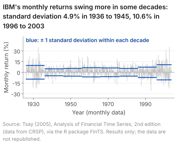
Large moves come in clusters: -22.6% in September 2002 was followed by +35.4% in October. Yet the returns themselves are almost uncorrelated with the month before (0.035, section 4). Their sizes are not. Take each month's distance from the mean return, ignoring its sign: the correlation between one month's distance and the next is 0.197. Large moves of either sign follow large moves, and calm months follow calm months: this is volatility clustering. Lesson 24 uses the same returns to separate "uncorrelated" from "independent", and the page on GARCH volatility models a spread that changes.
6. Outliers and shifts in the mean
An outlier is an observation far from the rest of the series; a shift in the mean is a change in the level the series moves around. Two quarters of 2020 show what an outlier does to the statistics of GDP growth, and inflation shows what a shift does to a mean.
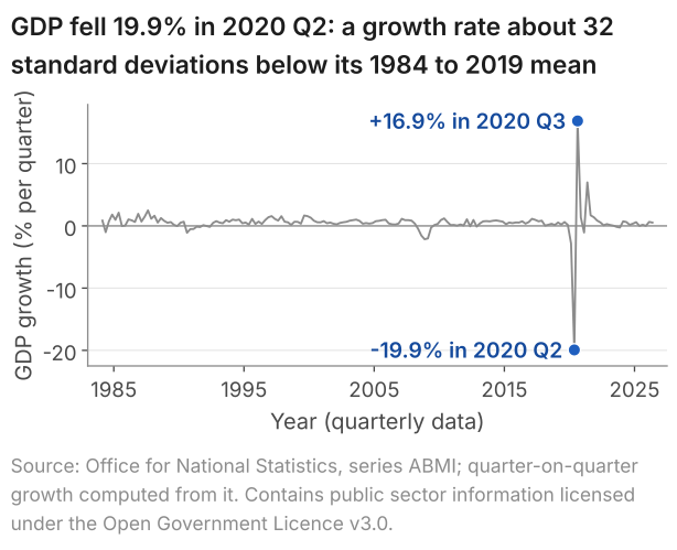
Figure 6 extends GDP growth to 2026 Q2. In standard deviations of the 1984 to 2019 quarters, the fall in 2020 Q2 lies about 32 below their mean: \((-19.9 - 0.56)/0.64 \approx -32\).
| GDP growth | 1984 Q1 to 2019 Q4 | 1984 Q1 to 2026 Q2 |
|---|---|---|
| Quarters, T | 144 | 170 |
| Mean (% a quarter) | 0.56 | 0.53 |
| Standard deviation | 0.64 | 2.18 |
| Correlation of one quarter's growth with the next | 0.56 | -0.27 |
Adding the 26 quarters from 2020 Q1 barely moves the mean, more than triples the standard deviation and turns the correlation between neighbouring quarters negative. Two quarters do nearly all of this. Their fall and rise nearly cancel in the mean, but the standard deviation adds up squared distances from the mean, which do not cancel: 2020 Q2 and Q3 make up 85% of the sum of squared deviations, and without them the other 168 quarters have a standard deviation of 0.85. And the fall followed at once by the rise puts two neighbours far apart on opposite sides of the mean: that one pair turns the correlation negative.
These quarters are data, not errors: GDP did fall by about a fifth in 2020 Q2. They are left out of the main sample because two quarters would otherwise dominate every statistic computed from it. Lesson 25 asks what a model fitted before 2020 would have forecast for 2020 Q2.
A shift in the mean is slower: the series settles around a new level. The table gives means and standard deviations in separate windows.
| Series and window | T | Mean (%) | Std. dev. |
|---|---|---|---|
| CPI inflation, January 1989 to December 1992 | 48 | 6.01 | 1.66 |
| CPI inflation, January 1993 to December 2019 | 324 | 2.04 | 0.99 |
| CPI inflation, January 2020 to August 2026 | 80 | 4.16 | 3.11 |
| GDP growth, 1984 Q1 to 2001 Q4 | 72 | 0.69 | 0.66 |
| GDP growth, 2002 Q1 to 2019 Q4 | 72 | 0.43 | 0.61 |
Inflation averaged 6.01% in its first four years, 2.04% over the next 27 and 4.16% since 2020, when its standard deviation also more than tripled. The mean of all 452 months, 2.84%, lies below the first window's mean, above the second's and below the third's: when the mean shifts, no single number describes the level of the series. GDP growth averaged 0.69% a quarter in the first half of the main sample and 0.43% in the second, which contains the recession of 2008 and 2009. Two cautions apply: a split chosen after looking at the graph makes a difference easier to find, and in a persistent series a mean over 72 quarters is less precise than 72 independent observations would make it (lesson 21). A mean or a spread that changes across the sample is evidence against stationarity, which lesson 24 defines and checks.
7. What a graph cannot settle
Eye-balling the graph of a series does not tell us the exact form of the process that produced it, nor does it give a framework for testing one model against another. In Figure 7 one series is the shocks themselves, independent from one period to the next; the other is built from the same shocks and has memory. Try to say which is which before reading the caption.
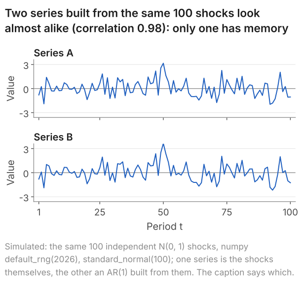
The eye does not separate them, and in this run neither does the count of section 4: Series B, the one with memory, has fewer than half its pairs on the same side of its mean. The correlation between one value and the next points the right way, 0.072 against 0.285, but in 100 values it is noisy: B's 0.285 lies above the 0.2 its rule implies, by chance in this run. So a graph cannot settle which process produced a series, nor whether a feature such as the gap between two window means is more than chance. Those questions need numbers whose chance error is known. Lesson 23 measures dependence and shows how far the measure can be trusted, and lesson 24 states the stability one history must have before it can teach us about its process.
8. Describing a graph in an exam or a report
The checklist becomes a written description once, for each feature, you say what you see, in which direction, and the evidence: in an exam, what you can read off the graph; in a report, a number.
| Feature | What to say | Example from this lesson |
|---|---|---|
| Trend | Up, down or none; in the level or the growth rate | GDP level 4.98 times its 1955 value; growth flat around 0.60% a quarter |
| Seasonality | High and low months; adjusted or not | Retail sales, not adjusted: December +25.8%, January -10.5% |
| Persistence | Sign and strength of the dependence | Unemployment: 660 of 664 pairs on the same side of the mean |
| Volatility | When the spread is wide or narrow | IBM: 4.9% in 1936 to 1945, 10.6% in 1996 to 2003 |
| Outliers | Dates and sizes; results with and without | GDP growth, 2020 Q2: -19.9%, about 32 standard deviations below the mean |
| Shift in the mean | When, and from what level to what | CPI inflation: 6.01% in 1989 to 1992, 2.04% in 1993 to 2019 |
A model description of the growth panel of Figure 1, in five sentences:
9. Common mistakes
When I marked answers to an exam question that asked for the features of a time-series graph, marks were lost for saying the data looked non-stationary without saying why, and for commenting on the dependence without giving its sign.
- "The data look non-stationary." Say what changes and by how much: the mean of inflation is 6.01% in 1989 to 1992 and 2.04% in 1993 to 2019.
- "There is dependence." Give its sign: positive for long spells on one side of the mean (unemployment, 4 crossings in 664 pairs), negative for a zigzag (the \(\phi = -0.9\) path of Figure 4, 83 crossings in 99 steps).
- Reading a December jump as news. December is the highest month of the unadjusted retail index in all 30 years: compare a December with earlier Decembers, or use an adjusted series.
- Dropping an outlier without a word. Give results with and without it: the standard deviation of GDP growth is 0.64 without the quarters from 2020 and 2.18 with them.
- "The graph shows which model fits." In Figure 7 a series with memory and one without look almost alike.
10. Check your understanding
Five questions, marked on the page; every option has an explanation, including the wrong ones. (Without JavaScript the explanations are shown beneath each question.)
1. Figure 5 marks plus and minus one standard deviation of IBM's monthly returns within each decade: 9.5% in 1926 to 1935, 4.9% in 1936 to 1945 and 10.6% in 1996 to 2003. The decade means of the returns lie between 0.11% and 2.15% a month. Which feature of the series do the bars show?
Correct. The bars measure the spread of the returns within each decade, and it more than doubles, from 4.9% in 1936 to 1945 to 10.6% in 1996 to 2003 (10.6/4.9 = 2.2). The level does not trend: the decade means stay between 0.11% and 2.15% a month.
The bars show widths, not levels. A trend would be a rising mean, and the decade means go up and down between 0.11% and 2.15% a month, with 2.14% in 1926 to 1935 and 2.07% in 1996 to 2003. What changes is the spread, from 4.9% to 10.6%.
Wide swings are not long spells. Persistence concerns the order of the values, and IBM's returns are on the same side of their mean as the month before in 472 of 935 pairs, 50.5%, about what independent values would give.
2. The four paths of Figure 4 share the same 100 shocks. Over its 99 steps, one of the paths crosses zero 83 times. What do the 83 crossings show about the dependence of each value on the one before?
Independent values symmetric about zero change sign on half the steps on average: 99/2 = 49.5 times in 99 steps. This path changes sign on 83 of its 99 steps, far more than that, so its values are not independent: the dependence is negative.
Correct. Independent values symmetric about zero would change sign on about half the steps, 49.5 of 99. This path changes sign on 83 because each value carries -0.9 times the one before: a value above zero is followed by one below unless the new shock outweighs the part carried over.
Positive dependence keeps a path on one side of zero: the \(\phi = 0.9\) path of the same figure crosses only 16 times. Swings across zero on 83 of 99 steps show negative dependence.
3. In 2005 the twelve monthly values of the retail sales index of Figure 2, which is not seasonally adjusted, have a mean of 54.4. November's value is 59.8 and December's 69.7. How far above its year's mean is December, as a percentage of that mean?
69.7 - 54.4 = 15.3 is the excess in index points, not in per cent. As a percentage of the year's mean it is 15.3/54.4 = 0.281, that is 28.1%.
69.7/59.8 = 1.166 compares December with November, the month before. The question compares December with the mean of its own year: 69.7/54.4 = 1.281, so 28.1% above it.
15.3/69.7 = 0.220 divides the excess by December's own value. The base is the year's mean: 15.3/54.4 = 0.281, so 28.1%.
Correct. December's ratio to the mean of its year is 69.7/54.4 = 1.281, so December is 28.1% above that mean. The average December excess over 1996 to 2025 is 25.8%; over 1996 to 2005 it is 28.1%, a ratio of 1.281.
4. UK real GDP, as published in September 2026, was £740.509 billion in 2026 Q1 and £744.453 billion in 2026 Q2 (chained volume measures, seasonally adjusted). What was growth in 2026 Q2 on the quarter before?
Correct. Growth = 100 × (744.453/740.509 - 1) = 100 × 0.00533 = 0.53%: the change, £3.944 billion, as a percentage of the level in the quarter before.
4 × 0.5326 = 2.13 multiplies the quarterly rate by four, as if it were growth over a year. The question asks for growth on the quarter before: 100 × (744.453/740.509 - 1) = 0.53%.
744.453 - 740.509 = 3.944 is the change in £ billion, not a growth rate. As a percentage of the level before it, 100 × 3.944/740.509 = 0.53%.
100 × 744.453/740.509 = 100.53 says that GDP in 2026 Q2 is 100.53% of its level in 2026 Q1. Growth is the change, so subtract 100: 0.53%.
5. A student looks at Figure 7 and says that Series A and Series B are both independent shocks, since neither shows any pattern. In fact Series B is built from Series A by \(Y_t = 0.2\,Y_{t-1} + \varepsilon_t\). What does the figure show?
Series B depends on its own past by construction: each value carries 0.2 of the one before. That it looks like A shows a limit of the eye, not an absence of memory. The correlation between one value and the next is 0.285 for B against 0.072 for A.
0.98 is the correlation between the two series at the same date, high because B is built from A's shocks. Memory is the dependence of a series on its own past, and A, the shocks themselves, has none by construction.
Correct. Series B carries 0.2 of each value into the next, yet in 100 values it looks like A, and even the count of pairs on the same side of the mean does not separate them: 47 of 99 for B, 43 for A. A graph cannot settle which process produced a series.
11. Three questions about time-series graphs
Look for six features: a trend, a pattern that repeats each year, persistence, a spread that changes over time, outliers and shifts in the mean. For each, say what you see, its direction and the evidence. UK unemployment shows persistence: it is on the same side of its mean as the value before in 660 of 664 pairs.
Seasonality is a pattern that repeats each year. UK retail sales, not seasonally adjusted, peak every December: from 1996 to 2025, December averaged 25.8% above the mean of its year and January 10.5% below. The pattern can drift: December's ratio to its year's mean averaged 1.281 in 1996 to 2005 and 1.231 in 2016 to 2025.
A seasonally adjusted series has had its pattern that repeats each year estimated and removed, so that neighbouring months or quarters can be compared. The Office for National Statistics publishes UK GDP and unemployment adjusted. The retail sales index used here is the unadjusted series, so it jumps every December, on average 25.8% above the mean of its year.
12. Where next
- Lesson 23: autocorrelation and the correlogram, which turns "looks persistent" into a number, computes it by hand and shows how far to trust it from one history.
- Lesson 24: stationarity, white noise and random walks, for what it means that a mean and a spread do not change, and what a trending series does to a regression.
- Time series econometrics notes, where the series of this lesson appear in one table with the feature each shows.
- Advanced time series notes, for models of seasonality, and GARCH volatility, for models of a spread that changes over time.
- The course home, which lists all 25 lessons and says which are published.
Stuck on describing a time-series graph? Send it
I tutor statistics and econometrics one-to-one, from a first confidence interval through to regression, panel data and time series. Bring the graph or the question you are stuck on and we will work through it in the free 30-minute consultation.
Book a free 30-minute consultation Econometrics tutor: how it works
Data and simulation. UK GDP: Source: Office for National Statistics, series ABMI (growth computed from ABMI), as published in September 2026. Contains public sector information licensed under the Open Government Licence v3.0. Retail sales: Source: Office for National Statistics, series J5AH. Contains public sector information licensed under the Open Government Licence v3.0. Unemployment: Source: Office for National Statistics, series MGSX. Contains public sector information licensed under the Open Government Licence v3.0. CPI inflation: Source: Office for National Statistics, series D7G7. Contains public sector information licensed under the Open Government Licence v3.0. The ONS series were retrieved on 10 October 2026. IBM: Source: Tsay (2005), Analysis of Financial Time Series, 2nd edition (data from CRSP), via the R package FinTS. Results only; the data are not republished. Figures 4 and 7, simulated: Y(t) = \(\phi\) Y(t-1) + e(t), e(t) independent N(0, 1), Y(0) = 0, T = 100, with \(\phi\) = 0.9, 0.2, -0.2 and -0.9; the same 100 shocks in every panel, from a fresh numpy default_rng(2026), standard_normal(100). Series A of Figure 7 is the shocks themselves and Series B the \(\phi\) = 0.2 path. The expected numbers of crossings are exact for a path started at 0, and were checked against 10,000 paths drawn with another fresh default_rng(2026), standard_normal((10000, 100)). Adapted from my lecture notes for Time Series Econometrics (ECON30401) at the University of Manchester.