
Among 1,388 births, a single birthweight lies a typical distance of about 20 ounces from their mean. The sample mean, 118.70 ounces, estimates the population mean and would vary from sample to sample by about half an ounce. The standard deviation measures the first spread, that of the data; the standard error the second, that of an estimate across samples.
In this lesson
- Two questions, two spreads: the comparison table
- The standard deviation describes the data
- Where the standard error comes from
- See it: 10,000 samples at seven sample sizes
- Four times the data halves the standard error
- Which one to report, and how to read error bars
- Every estimate has a standard error
- Common mistakes
- Check your understanding: five marked questions
- Three questions about standard errors
- Where next
1. Two questions, two spreads
A set of data raises two questions about spread, and each has its own measure. The 1988 National Health Interview Survey in the United States recorded the birthweights of 1,388 babies, and their mean is 118.70 ounces. Lesson 4 treated these births as a population to draw samples from. Here they are a sample from the population of births the survey was drawn from.
Question 1: how far does one baby's weight lie from the mean? A typical distance is 20.35 ounces. This is the standard deviation of the 1,388 weights, which we write \(s\). It describes the data.
Question 2: how far does the sample mean lie from the population mean? The population mean is unknown, so for our own sample we cannot say. What one sample can estimate is the typical distance between a sample mean and the population mean, across all the samples of 1,388 births that might have been drawn: 0.546 ounces. This is the standard error of the sample mean, \(s/\sqrt{n}\), where \(n = 1{,}388\) is the number of observations. It describes the estimate.
The table sets the two side by side.
| Standard deviation | Standard error | |
|---|---|---|
| What it measures | How far single observations lie from their mean | How far an estimate lies from the population value, across samples |
| What it describes | The data | An estimate, such as the sample mean |
| How it is computed | \(s\), from the squared distances from the mean | \(s/\sqrt{n}\) for a sample mean |
| As the sample grows | Settles near the population standard deviation | Falls towards zero |
| Where it appears | Tables of summary statistics | Beside an estimate, or in brackets under a regression coefficient |
| Units | Those of the data | Those of the estimate; for a mean, those of the data |
| The 1,388 births | 20.35 ounces | 0.546 ounces |
The population mean \(\mu\) and standard deviation \(\sigma\) are fixed numbers that we do not know; \(s\) estimates \(\sigma\). We write \(\bar X\) for the sample mean as it varies from sample to sample, and \(\bar x\) for its value in our sample, 118.70, following lesson 2: a capital letter for what varies, the lower-case letter for the value observed. Books use other letters; the choice is cosmetic.
What students say
“Nicky is an excellent econometrics tutor. He explains complex concepts clearly and makes them much easier to understand.”
“I was completely lost in my economics class, and then I started working Nicky and he totally saved me. He was excellent at explaining the material and extremely accommodating to meet with me many times despite us being in different time zones! Highly recommend working with Nicky!”
“Nicky is a very good and thorough teacher. He has excellent knowledge of econometrics and takes the time to work through your questions. Highly recommended!”
“Really great tutor! Encouraging, knowledgeable, friendly”
“Very good lesson, Nicky is very helpful.”
“Very helpful and clear.”
“I gather it was very useful, thank you!”
“Fantastic!”
2. The standard deviation describes the data
The standard deviation measures how far single observations lie from their mean. Each observation's distance from the sample mean is squared, so that distances above and below do not cancel. The squares are added and divided by \(n - 1\), and the square root takes the result from ounces squared back to ounces:
$$ s = \sqrt{\frac{1}{n-1}\sum_{i=1}^{n}(x_i - \bar x)^2} . $$In words: standard deviation = square root of (the sum of squared distances from the mean, divided by n - 1).
Squared distances from \(\bar x\) add up to no more than squared distances from the unknown \(\mu\) would, in every sample, and dividing by \(n - 1\) rather than \(n\) makes up for that on average: under random sampling, \(s^2\) is right on average for \(\sigma^2\) (lesson 3). The result estimates \(\sigma\), the standard deviation of birthweight in the population: \(s = 20.35\) ounces for the 1,388 births.
Because \(\sigma\) is a fixed feature of the population, more data do not make \(s\) smaller; they make it a better estimate of the same number. The births, in the order of the data set, show this. Each set in the table contains the one before, so these are not independent samples.
| Births used | First 25 | First 100 | First 400 | All 1,388 |
|---|---|---|---|---|
| Standard deviation (oz) | 22.22 | 17.61 | 20.75 | 20.35 |
The standard deviation moves from 22.22 to 17.61 to 20.75 and ends at 20.35: it settles near 20 ounces rather than shrinking.
3. Where the standard error comes from
What we are after. We want the typical distance between the sample mean \(\bar X\) and the population mean \(\mu\), across all the samples of \(n\) births we might have drawn. Under random sampling, meaning that each observation is drawn independently from the same population, the sample mean is centred on \(\mu\): across samples it is neither too high nor too low on average, as lesson 4 shows. So what remains to measure is how widely \(\bar X\) is spread around \(\mu\).
The measure. It is the variance of the sample mean: the average squared distance between the sample mean and the population mean, taken over all the samples we could have drawn. In symbols, \(\operatorname{Var}(\bar X) = E[(\bar X - \mu)^2]\), where \(E\), the expectation, is here the average over samples. Squaring keeps distances above \(\mu\) and below it from cancelling.
The assumption, and what it gives. Under random sampling, from a population whose variance \(\sigma^2\) is finite,
$$ \operatorname{Var}(\bar X) = \frac{\sigma^2}{n} . $$In words: variance of the sample mean = variance of one observation divided by the number of observations.
Show where \(\sigma^2/n\) comes from
- The sample mean is a scaled sum. \(\bar X = \frac{1}{n}(X_1 + X_2 + \dots + X_n)\), where \(X_1, \dots, X_n\) are the \(n\) observations before the sample is drawn.
- The constant comes out squared. Multiplying a random variable by a constant \(a\) multiplies its variance by \(a^2\). Here \(a = 1/n\), so $$ \begin{aligned} &\operatorname{Var}(\bar X) \\ &= \frac{1}{n^2}\operatorname{Var}(X_1 + \dots + X_n) . \end{aligned} $$
- Independence removes the covariances. The variance of a sum is the sum of the variances plus twice the covariance of every pair. Under random sampling the observations are independent, so every covariance is zero. Each observation has variance \(\sigma^2\), so the sum has variance \(n\sigma^2\).
- Combine the two. $$ \operatorname{Var}(\bar X) = \frac{n\sigma^2}{n^2} = \frac{\sigma^2}{n} . $$
The two rules for variances are in lesson 3. Lesson 4 checks the result against 10,000 simulated samples.
The derivation uses independence and the fact that every observation has variance \(\sigma^2\), and nothing about the sample size or the shape of the population. So \(\sigma^2/n\) holds for every \(n\), not only in large samples.
Why divide by \(n\). Intuitively, the larger the sample, the more closely it resembles the population it was drawn from, and so the less one sample can differ from another by chance. A single birth can lie a long way from the mean: 13 of the 1,388 lie more than 60 ounces from it. In a sample of 25 the unusually heavy and the unusually light babies largely offset one another, so the mean of 25 strays far less. Figure 1 shows this, treating the 1,388 births, as lesson 4 did, as the whole population and drawing 10,000 samples of 25 from them.
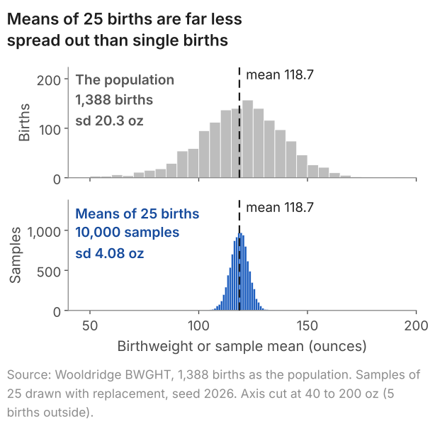
As \(n\) increases, the mix of values in the sample comes closer to the mix in the population, the random variation in its mean decreases, and \(\sigma^2/n\) falls towards zero. It is above zero at every sample size: however large the sample, another random sample of the same size could give a different mean.
Why the square root. A variance is an average of squared distances, so \(\sigma^2/n\) is in squared units: ounces squared for the births. Taking the square root returns it to ounces, the units the data are measured in, so that it can be read as a typical distance between the sample mean and the population mean:
$$ \sqrt{\operatorname{Var}(\bar X)} = \frac{\sigma}{\sqrt{n}} . $$In words: standard deviation of the sample mean = standard deviation of one observation divided by the square root of the number of observations.
Strictly, this typical distance is the square root of the average squared distance, not the average distance. For a normal distribution the average distance is \(\sqrt{2/\pi} = 0.80\) times the standard deviation, so the two are on the same scale as well as in the same units. The 10,000 means of Figure 1 lie on average 3.24 ounces from the centre, against a standard deviation of 4.08.
From \(\sigma\) to \(s\). The population standard deviation \(\sigma\) is unknown, so we estimate it by the sample standard deviation \(s\). The result is the standard error of the sample mean: our estimate, from the one sample we have, of the standard deviation of the sample mean across samples. For the births,
$$ \text{se}(\bar X) = \frac{s}{\sqrt{n}} = \frac{20.35}{\sqrt{1388}} = 0.546 \text{ ounces.} $$In words: standard error of the mean = standard deviation of the data divided by the square root of the number of observations.
Definition: standard error
The standard error of an estimate is the standard deviation of that estimate across repeated samples: for the sample mean, \(\sigma/\sqrt{n}\). When the population values it depends on are unknown, it is estimated from the one sample in hand, and the estimate goes by the same name: for the sample mean, \(\text{se}(\bar X) = s/\sqrt{n}\), with \(s\) the sample standard deviation and \(n\) the number of observations.
Remarks. In words: the standard error is the typical distance between an estimate and the population value across repeated samples. It describes the estimate, not the data. The weights of the 1,388 babies spread by 20.35 ounces; their mean, by 0.546.
One name, two cases. Is the standard error a population quantity or a sample one? This course uses the name for both. When \(\sigma\) is known, \(\sigma/\sqrt{n}\) is the standard error, known rather than estimated: the first examples of lessons 7 and 8 work this way, with \(\sigma = 10\) marks and a standard error of 2. When \(\sigma\) is unknown, as it is for the births, the standard error is \(s/\sqrt{n}\), itself an estimate that changes from sample to sample with \(s\); this is what software prints. For grades like these, \(s/\sqrt{25}\) came out between 1.52 and 2.46 marks in 90% of 10,000 simulated samples of 25, around \(\sigma/\sqrt{25} = 2\). Some books keep the name for the second case and call \(\sigma/\sqrt{n}\) the standard deviation of the sample mean. The difference is in the name only.
4. See it: the standard deviation stays put, the standard error shrinks
The two spreads behave differently as \(n\) grows. Take first exam grades, normally distributed with standard deviation \(\sigma = 10\) marks, as in lessons 6 to 8. For samples of 25, the variance of the sample mean is \(\sigma^2/n = 100/25 = 4\) marks squared, and its square root is 2 marks: one grade lies a typical 10 marks from the population mean, the mean of 25 grades a typical 2.
To watch both spreads change, we drew \(R = 10{,}000\) samples from such a population, with mean 65, at each of seven sample sizes \(n\) from 1 to 400 (\(R\) counts the samples, \(n\) the observations in each). At each size we took the standard deviation of the 10,000 sample means and the average of the 10,000 sample standard deviations. Figure 2 plots both against \(n\); the table gives the numbers.
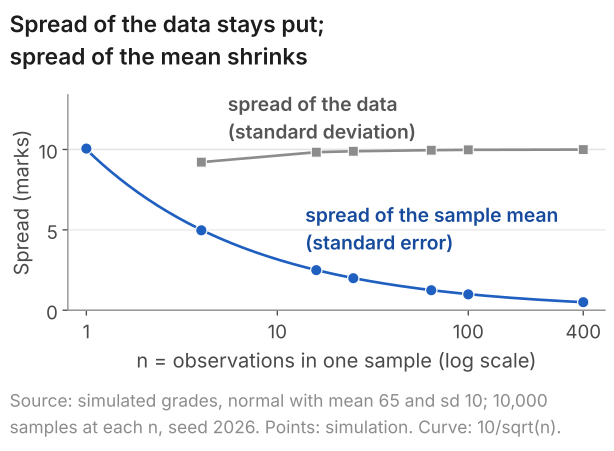
| n | Std. deviation of the 10,000 sample means | 10/√n | Average s |
|---|---|---|---|
| 1 | 10.057 | 10.000 | none |
| 4 | 4.971 | 5.000 | 9.21 |
| 16 | 2.492 | 2.500 | 9.83 |
| 25 | 1.991 | 2.000 | 9.89 |
| 64 | 1.243 | 1.250 | 9.96 |
| 100 | 0.985 | 1.000 | 9.98 |
| 400 | 0.500 | 0.500 | 9.99 |
Down the second column the spread of the sample mean follows 10/√n, from 10 marks for single grades to half a mark for means of 400. Down the last, the average standard deviation of the data does not fall; it rises slightly and settles near 10, the population value (one grade has no standard deviation). Dividing by \(n - 1\) makes \(s^2\) right on average, but the square root of an average exceeds the average of the square roots, so \(s\) itself averages a little below 10 in small samples: 9.21 at \(n = 4\) (lesson 3).
Real data behave the same way. Treated again as a population, the 1,388 births have standard deviation \(\sigma = 20.347\) ounces (computed with divisor 1,388, the population's size, not 1,387). Samples of 25, 100 and 400 drawn from them with replacement, 10,000 of each, give means with standard deviations of 4.08, 2.04 and 1.04 ounces, against \(\sigma/\sqrt{n}\) = 4.07, 2.03 and 1.02. Drawing with replacement keeps the draws independent, as \(\sigma/\sqrt{n}\) requires; samples of 400 drawn without replacement, each holding 29% of the births, would have means with a smaller standard deviation, about 0.86 ounces.
Two simulated figures sit further from the formula than the rest: 0.985 against 1 for the grades at \(n = 100\), and 1.04 against 1.02 for the births at \(n = 400\). A standard deviation computed from 10,000 simulated means is itself an estimate, with a standard error of about 0.7% of its size here. These two lie 2.1 and 2.5 of those standard errors from the formula, gaps that chance alone produces in about 4% and 1% of simulations. The seed was not changed to remove them.
5. Four times the data halves the standard error
The variance of the sample mean, \(\sigma^2/n\), falls in proportion to \(1/n\), so its square root falls in proportion to \(1/\sqrt{n}\): precision grows with the square root of the sample size, not with the sample size itself. Hence halving the standard error takes four times the data, and cutting it to a tenth takes a hundred times.
In the table of section 4, \(10/\sqrt{n}\) falls from 2 marks to 1 as \(n\) goes from 25 to 100, and from 1 to 0.5 as it goes from 100 to 400. For the births, halving 0.546 ounces to 0.273 would take \(4 \times 1{,}388 = 5{,}552\) births, if their standard deviation stayed near 20.35: \(20.35/\sqrt{5552} = 0.273\). A tenth, 0.055 ounces, would take 138,800 births.
The first observations buy far more precision than later ones. With \(\sigma = 10\), the first hundred grades take the standard deviation of the mean from 10 marks (one grade) to 1 mark; the next hundred take it only from 1 to 0.71.
6. Which one to report, and how to read error bars
Software prints both the standard deviation and the standard error. For the 1,388 births:
| n | Mean (oz) | Std. deviation | Std. error | 95% interval |
|---|---|---|---|---|
| 1,388 | 118.70 | 20.35 | 0.546 | 117.63 to 119.77 |
Stata: the code
* once: ssc install bcuse
bcuse bwght, clear
summarize bwght
ci means bwght
Stata: what it prints
. summarize bwght

    Variable |        Obs        Mean    Std. dev.       Min        Max
-------------+---------------------------------------------------------
       bwght |      1,388    118.6996    20.35396         23        271

. ci means bwght

    Variable |        Obs        Mean    Std. err.       [95% conf. interval]
-------------+---------------------------------------------------------------
       bwght |      1,388    118.6996     .546329        117.6278    119.7713
R: the code
# birth weights (ounces), 1,388 babies: mean, sd, se, 95% interval
library(wooldridge)
data("bwght")
x <- bwght$bwght
length(x)
mean(x)
sd(x)
sd(x) / sqrt(length(x))
t.test(x)$conf.int
R: what it prints
> # birth weights (ounces), 1,388 babies: mean, sd, se, 95% interval
> library(wooldridge)
> data("bwght")
> x <- bwght$bwght
> length(x)
[1] 1388
> mean(x)
[1] 118.6996
> sd(x)
[1] 20.35396
> sd(x) / sqrt(length(x))
[1] 0.546329
> t.test(x)$conf.int
[1] 117.6278 119.7713
attr(,"conf.level")
[1] 0.95
Python: the code
import wooldridge
from scipy import stats

# birth weights (ounces), 1,388 babies: mean, sd, se, 95% interval
bwght = wooldridge.data("bwght")["bwght"]
n = len(bwght)
mean = bwght.mean()
se = stats.sem(bwght)
print("n:", n)
print("mean:", mean)
print("standard deviation:", bwght.std())
print("standard error:", se)
low, high = stats.t.interval(0.95, df=n - 1, loc=mean, scale=se)
print("95% interval:", low, high)
Python: what it prints
n: 1388
mean: 118.69956772334294
standard deviation: 20.353964337903857
standard error: 0.5463290277237868
95% interval: 117.62784728314541 119.77128816354046
The data set is Wooldridge's BWGHT, which the code loads; bwght is birthweight in ounces. The 95% interval is the subject of lesson 6.
Report the standard deviation when the point is how varied the individuals are. Report the standard error, or the confidence interval built from it in lesson 6, when the point is how precisely a population value has been estimated.
Figure 3 draws the means of two groups three times: babies whose mothers did not smoke during pregnancy (1,176 births) and babies whose mothers smoked (212). The bars are plus and minus one standard deviation, plus and minus one standard error, and the 95% confidence interval.
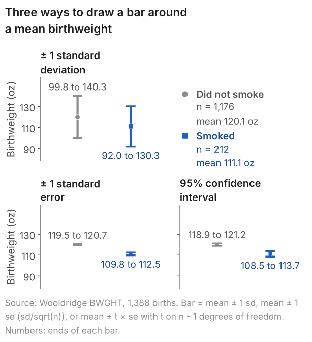
Individual weights in the two groups overlap heavily, so the standard deviation bars overlap over 30 ounces, from 99.8 to 130.3. Each mean, though, is estimated precisely, and the two means differ by 8.9 ounces, so the standard error bars and the 95% intervals do not overlap: the intervals are 5.2 ounces apart. Neither picture is wrong: they answer different questions, so a bar on a chart has to say what it is. The comparison is an association: on its own it does not show that smoking caused the difference.
The smokers' mean rests on 212 births against 1,176, and \(\sqrt{1176/212} = 2.36\). So their standard error, 1.317, is more than twice the non-smokers' 0.591, although their standard deviation is the smaller of the two, 19.18 against 20.27.
7. Every estimate has a standard error
The standard error is not special to the sample mean. Any estimate computed from a sample varies from one sample to the next, and its standard error is its standard deviation across samples, estimated from the sample in hand. Each estimate has its own formula, built by the steps of section 3.
A proportion. 212 of the 1,388 mothers smoked during pregnancy, a share of 0.153. A share is a mean: code each mother 1 if she smoked and 0 if not, and the share is the sample mean \(\bar x\) of the 0/1 values. In the population the 0/1 variable has mean \(p\), the population share, and variance \(p(1 - p)\) (lesson 3). Under random sampling, as for any mean, the variance of the sample share is that variance divided by \(n\). We do not know \(p\), so, as with \(s\) for \(\sigma\), we put the sample share in its place: the standard deviation of the 0/1 values becomes \(\sqrt{0.153 \times 0.847} = 0.360\), and dividing by \(\sqrt{n}\) gives the standard error of the share:
$$ \begin{aligned} \text{se}(\bar X) &= \sqrt{\frac{\bar x(1 - \bar x)}{n}} \\ &= \sqrt{\frac{0.153 \times 0.847}{1388}} = 0.0097 . \end{aligned} $$In words: standard error of a share = square root of (share times one minus the share, divided by the number of observations).
In another sample of 1,388 births, the share of mothers who smoked would differ from the population share by a typical distance of about one percentage point.
A regression slope. Regressing birthweight on the mother's cigarettes a day gives a slope of -0.514 ounces per cigarette: each extra cigarette a day goes with a birthweight about half an ounce lower. Its standard error is 0.0905 ounces per cigarette. That is not the standard deviation of birthweight (20.35 ounces) or of cigarettes a day (5.97), and it is not either of them divided by \(\sqrt{1388}\) (0.546 and 0.160). It has a formula of its own, built from the variance of the slope across samples, which lesson 11 works out from the residuals.
8. Common mistakes
- Using the standard deviation where the standard error belongs. \(118.70 \pm 1.96 \times 20.35\) runs from 78.8 to 158.6 ounces and holds 1,321 of the 1,388 babies: it describes babies, not the mean. An interval for the mean uses 0.546.
- Expecting the standard deviation to fall as the sample grows. It settles: 22.22, 17.61, 20.75 and 20.35 for the first 25, 100, 400 and all 1,388 births. The standard error is what falls.
- Dividing by \(n\) in place of \(\sqrt{n}\). \(20.35/1388 = 0.0147\). The standard error divides by \(\sqrt{1388} = 37.3\), not by 1,388, and is 0.546.
- Dividing by \(\sqrt{n}\) twice. The standard deviation of a set of simulated sample means already estimates the standard error: 1.99 marks for 10,000 means of 25 grades. Dividing by \(\sqrt{25}\) again gives 0.40, a fifth of the right answer.
- Reading the standard error as the spread of the data. "Birthweights vary by about half an ounce" is wrong: they vary by about 20 ounces. The 0.546 describes the mean.
- An error bar with no label. In Figure 3 the same data give bars about 20 ounces either side of a mean, or 0.6 to 1.3. Say which.
- "The standard error is always smaller than the standard deviation." For the mean of two or more observations that are not all equal, \(\sqrt{n}\) is above 1, so \(s/\sqrt{n}\) is below \(s\). For a slope the standard error is in ounces per cigarette, and a comparison with a standard deviation in ounces has no meaning.
9. Check your understanding
Five questions, marked on the page; every option has an explanation, including the wrong ones. (Without JavaScript the explanations are shown beneath each question.)
1. A random sample of 64 students has a mean grade of 61 marks and a standard deviation of 12 marks. What is the standard error of the sample mean?
12/64 = 0.19 divides by n. The standard error divides by the square root of n: 12/√64 = 12/8 = 1.5 marks.
Correct. The standard error of a mean is s/√n = 12/√64 = 12/8 = 1.5 marks: the typical distance between the mean of 64 grades and the population mean, across samples.
12²/64 = 144/64 = 2.25 is the variance of the sample mean, in marks squared. The standard error is its square root, √2.25 = 1.5 marks.
12 marks is the standard deviation of single grades. The mean of 64 grades varies far less from sample to sample: 12/√64 = 1.5 marks.
2. A table of summary statistics for the hourly wages of 526 workers (Wooldridge's WAGE1, 1976) reports a mean of $5.90, a standard deviation of $3.69 and a standard error of $0.161. One worker earns $9.59. Which statement about that wage is right?
Correct. How far one worker's wage lies from the mean is measured by the standard deviation: (9.59 - 5.90)/3.69 = 1.0. In these data 70 of the 526 workers, 13%, earn more than $9.59.
The arithmetic is right, (9.59 - 5.90)/0.161 = 22.9, but the standard error, $0.161, is the spread of the mean of 526 wages across samples, not of single wages. It says nothing about how many workers earn more than $9.59: 70 of the 526 do.
5.90 ± 1.96 × 0.161 = 5.58 to 6.22 is a 95% confidence interval for the population mean wage, not a range for single wages: only 36 of the 526 wages lie inside it.
3. From 100 grades a researcher finds a standard deviation of 10 marks and a standard error of the mean of 1 mark. She adds 300 grades from the same population, 400 in all. What should she expect the two numbers to be now?
The standard deviation describes single grades, and adding grades does not make them less spread out: it settles near 10. Only the standard error falls, to about 10/√400 = 0.5.
Quartering the standard error would need it to fall in proportion to 1/n. Four times the data quarters the variance of the mean, from 1 to 0.25 marks squared; the standard error, its square root, halves to 0.5.
Correct. The standard deviation estimates the spread of single grades in the population, which more data do not change: in lesson 5's simulation of grades with standard deviation 10, its average is 9.98 at n = 100 and 9.99 at n = 400. The standard error falls to about 10/√400 = 0.5.
4. In WAGE1 (1976), the 252 women have a mean hourly wage of $4.59 with a standard deviation of $2.53, and the 274 men $7.10 with $4.16. A chart draws each mean with a bar that is not labelled: $4.43 to $4.75 for the women and $6.85 to $7.35 for the men. What are the bars?
Correct. The bars reach about 0.16 and 0.25 either side of the means, and those are the standard errors: 2.53/√252 = 2.53/15.87 = 0.159 and 4.16/√274 = 4.16/16.55 = 0.251.
Bars of one standard deviation would run from 4.59 - 2.53 = 2.06 to 7.12 for the women and from 2.94 to 11.26 for the men, far wider than these.
A 95% interval reaches about 1.96 standard errors either side: 4.28 to 4.90 for the women and 6.61 to 7.59 for the men. These bars reach one standard error, so they are narrower.
5. Over the 1,900 Premier League matches of 2019/20 to 2023/24 the home side won 838, a share of 0.441. Treat them as independent draws from the matches such sides could play, which is an approximation, since each club plays 38 a season. What is the standard error of the share?
0.441 × 0.559/1900 = 0.00013 is the variance of the share. The standard error is its square root, 0.0114.
Correct. A share is the mean of 0/1 values (1 for a home win), whose standard deviation is √(0.441 × 0.559) = 0.497. Dividing by √1900 = 43.59 gives 0.0114, a little over one percentage point.
√(0.441/1900) = 0.0152 takes the variance of a 0/1 value to be the share itself. It is 0.441 × 0.559 = 0.247, which gives √(0.247/1900) = 0.0114.
0.497 is the standard deviation of the 0/1 results of single matches. The share of 1,900 matches varies far less: 0.497/√1900 = 0.0114.
10. Three questions about standard errors
The standard deviation measures how far single observations lie from their mean; the standard error measures how far an estimate, such as the sample mean, lies from the population value across repeated samples. For 1,388 birthweights the standard deviation is 20.35 ounces and the standard error of their mean is 20.35/√1388 = 0.546 ounces.
Under random sampling, high and low values partly offset one another in an average, and the variance of the sample mean is the variance of one observation divided by n: σ²/n. Its square root returns it to the units of the data, σ/√n, and the sample's s replaces the unknown σ. For 1,388 birthweights, 20.35/√1388 = 0.546 ounces.
For a sample mean, yes, once there are two or more observations that are not all equal: √n is then above 1, so s/√n is below s. For 1,388 birthweights the standard error is 0.546 ounces against a standard deviation of 20.35. For a regression slope the standard error is in ounces per cigarette, so the comparison has no meaning.
11. Where next
- Lesson 6: confidence intervals, and what 95% means, where the standard error becomes an interval that contains the population mean in 95% of samples.
- Lesson 4: sampling distributions, the law of large numbers and the central limit theorem (previous), for the simulation behind \(\sigma^2/n\) and the shape of the distribution of the sample mean.
- Lesson 11: reading regression output, for the standard error of a regression coefficient.
- The course home, which lists all 25 lessons and says which are published.
Stuck on a standard error question? Send it
I tutor statistics and econometrics one-to-one, from a first standard error through to regression, panel data and time series. Bring the question you are stuck on and we will work through it in the free 30-minute consultation.
Book a free 30-minute consultation Econometrics tutor: how it works
Data and simulation. Birthweights: Wooldridge, Introductory Econometrics: A Modern Approach, data set BWGHT (1,388 births, 1988 National Health Interview Survey); "first 25", "first 100" and "first 400" are the first rows of the file; a smoker is a mother with at least one cigarette a day; results quoted, data not republished. Births treated as a population (Figure 1 and section 4): for each n in 25, 100 and 400, a fresh numpy default_rng(2026) and rng.choice(births, size=(10000, n), replace=True), where births holds the 1,388 weights in file order; one row per sample; Figure 1 shows the n = 25 draws. Grades (Figure 2 and section 4): an illustrative normal population with mean 65 and standard deviation 10; for each n in 1, 4, 16, 25, 64, 100 and 400, a fresh default_rng(2026) and rng.normal(65, 10, size=(10000, n)), one row per sample; standard deviation of the 10,000 means with divisor R - 1, sample standard deviations with divisor n - 1. Questions: Wooldridge WAGE1 (526 workers, 1976); Premier League results from openfootball/england (CC0), 1,900 matches, 2019/20 to 2023/24; the other question data are illustrative. Adapted from my lecture notes for the MSc pre-sessional statistics course (ECON60901, 2015 and 2016) and for Time Series Econometrics (ECON30401) at the University of Manchester, and for Financial Econometrics (EC5609) at the University of St Andrews.