
The sample mean is an estimate of the true population mean. Each sample is generally different, though, and hence each sample mean will vary. A confidence interval provides a method to quantify this sampling variation: a range around the sample mean, built to contain the true population mean with a stated probability across repeated samples, conventionally 95%.
In this lesson
- One sample, one estimate: 1,388 births
- How far the sample mean varies: the standard error
- From the standard error to an interval
- What the 95% means: 10,000 samples
- Where the multiple comes from, and why 1.96 fails in small samples
- An interval by hand: five workers
- Five real intervals: home advantage in the Premier League
- What makes an interval wider or narrower
- Common mistakes
- Check your understanding: five marked questions
- Three questions about intervals
- Where next
1. One sample, one estimate
The 1988 National Health Interview Survey in the United States recorded the birthweight of 1,388 babies. Their mean birthweight is 118.70 ounces, about 3.37 kilograms. Suppose we want to know the mean birthweight among all the births the survey was drawn from. The 1,388 are a sample from that population, so 118.70 is an estimate of the population mean. It is not the population mean itself.
Had the survey reached a different 1,388 mothers, the sample mean would have come out a little differently: 118.2, perhaps, or 119.1. So the single number 118.70 is not a complete answer. We also need to say how far a sample mean is likely to lie from the population mean. A confidence interval does that. It turns "118.70" into "118.70, with a margin of 1.07 either side", where the margin is built so that the interval contains the population mean in about 95% of samples.
The population mean, which we write \(\mu\), is a fixed number. We do not know it, but it does not change from sample to sample. The sample mean is what changes: each sample gives its own value. We write \(\bar X\) for the sample mean when we think of it as varying from sample to sample, and \(\bar x\) for the value it takes in the sample we have, here 118.70. (A capital letter for a quantity that varies from sample to sample and the lower-case letter for its observed value is the convention set out in lesson 2. Books differ in the letters they use, and the choice is cosmetic.) The margin comes from how far \(\bar X\) varies around \(\mu\).
What students say
“Nicky is an excellent econometrics tutor. He explains complex concepts clearly and makes them much easier to understand.”
“I was completely lost in my economics class, and then I started working Nicky and he totally saved me. He was excellent at explaining the material and extremely accommodating to meet with me many times despite us being in different time zones! Highly recommend working with Nicky!”
“Nicky is a very good and thorough teacher. He has excellent knowledge of econometrics and takes the time to work through your questions. Highly recommended!”
“Really great tutor! Encouraging, knowledgeable, friendly”
“Very good lesson, Nicky is very helpful.”
“Very helpful and clear.”
“I gather it was very useful, thank you!”
“Fantastic!”
2. How far the sample mean varies: the standard error
To quantify the sampling variation we need a measure of how far the sample mean \(\bar X\) lies from the population mean \(\mu\) across samples. We assume random sampling: each observation is drawn independently from the same population. Lesson 4 shows that under random sampling the sample mean is centred on \(\mu\): across samples it is neither too high nor too low on average. What remains is how widely it is spread around that centre. The measure is the variance of the sample mean: the average squared distance between \(\bar X\) and \(\mu\), taken over all the samples we could have drawn.
Under random sampling, if each observation has variance \(\sigma^2\) in the population, then
$$ \operatorname{Var}(\bar X) = \frac{\sigma^2}{n} . $$In words: variance of the sample mean = variance of one observation divided by the number of observations.
Show where \(\sigma^2/n\) comes from
- Write the sample mean as a sum. \(\bar X = \frac{1}{n}(X_1 + X_2 + \dots + X_n)\), where \(X_1, \dots, X_n\) are the \(n\) observations before they are drawn.
- Take the constant out. Multiplying a random variable by a constant \(a\) multiplies its variance by \(a^2\). Here \(a = 1/n\), so $$ \begin{aligned} &\operatorname{Var}(\bar X) \\ &= \frac{1}{n^2}\operatorname{Var}(X_1 + X_2 \\ &\qquad + \dots + X_n) . \end{aligned} $$
- Use random sampling. The observations are independent, and the variance of a sum of independent random variables is the sum of their variances. Each observation comes from the same population, so each has variance \(\sigma^2\), and the sum has variance \(n\sigma^2\).
- Put the two together. $$ \operatorname{Var}(\bar X) = \frac{n\sigma^2}{n^2} = \frac{\sigma^2}{n} . $$
The two rules for variances used in steps 2 and 3 are in lesson 3. Lesson 4 checks the result against 10,000 simulated samples.
Intuitively, the larger the sample, the more closely it resembles the population it was drawn from, and so the less one sample can differ from another by chance. A single birthweight can lie far from the mean: 13 of the 1,388 lie more than 60 ounces from it. In a mean of 1,388 birthweights the unusually heavy babies and the unusually light ones largely offset one another. As \(n\) increases the random variation in the sample mean decreases, and \(\sigma^2/n\) falls towards zero.
A variance is an average of squared distances, so it is measured in squared units, here ounces squared. Taking the square root returns it to ounces, the units the data are measured in, so that it can be read as a typical distance between the sample mean and the population mean: the square root of their average squared distance. The square root of \(\sigma^2/n\) is \(\sigma/\sqrt{n}\), the standard deviation of the sample mean.
We do not know \(\sigma\), because it is a feature of the population. We estimate it with the standard deviation of the sample, \(s\), which is 20.35 ounces for the birthweights. The result is the standard error of the sample mean, our estimate of its standard deviation across samples:
$$ \text{se}(\bar X) = \frac{s}{\sqrt{n}} = \frac{20.35}{\sqrt{1388}} = 0.546 \text{ ounces.} $$In words: standard error of the mean = standard deviation of the data divided by the square root of the number of observations.
The two numbers measure different spreads. A single birthweight lies about 20 ounces from the mean of the births, as a typical distance. The mean of 1,388 birthweights varies from sample to sample around the population mean by about half an ounce, on the same measure; how far our own 118.70 lies from the population mean we cannot know. Lesson 5 sets the standard deviation and the standard error side by side, and shows why four times the data halves the standard error.
3. From the standard error to an interval
An interval with a stated probability needs the shape of the distribution of the sample mean as well as its spread. Under random sampling, the distribution of the sample mean is approximately normal in large samples, whatever the shape of the population, provided its variance is finite. This is the central limit theorem of lesson 4. The distribution is centred on \(\mu\), and its standard deviation is the \(\sigma/\sqrt{n}\) of section 2, which the standard error estimates.
A normal distribution has 95% of its probability within 1.96 standard deviations of its centre. Hence, in a large sample, the sample mean lies within \(1.96\,\sigma/\sqrt{n}\) of the population mean in about 95% of samples; and since \(s\) is close to \(\sigma\) in a large sample (the law of large numbers), it lies within 1.96 standard errors of the population mean in about 95% of samples too.
A distance is the same in whichever direction it is measured. So whenever the sample mean is within 1.96 standard errors of \(\mu\), \(\mu\) is within 1.96 standard errors of the sample mean. It follows that the interval running 1.96 standard errors either side of the sample mean contains \(\mu\) in about 95% of samples. For the births:
$$ 118.70 \pm 1.96 \times 0.546 = 118.70 \pm 1.07 . $$That is, 117.63 to 119.77 ounces.
Definition: confidence interval for a mean
A 95% confidence interval for the population mean \(\mu\) is
$$ \bar x \;\pm\; c \times \frac{s}{\sqrt{n}} , $$where \(\bar x\) is the sample mean, \(s\) the sample standard deviation, \(n\) the sample size and \(c\) a multiple chosen so that intervals built in this way contain \(\mu\) in 95% of samples. In a large sample \(c = 1.96\), and intervals built with it contain \(\mu\) in about 95% of samples.
Remarks. The interval is centred on the estimate, and its half-width, \(c \times s/\sqrt{n}\), is called the margin of error. The two ends of the interval are computed from the sample, so they change from sample to sample. The population mean does not. Before the sample is drawn it is the interval that is random, and \(\mu\) that is fixed.
The same recipe on smaller samples shows what the interval is doing. Take only the first 25 births in the file, then the first 100, then all 1,388. The three samples overlap (the first 25 are among the first 100), so the rows show how one interval changes as births are added. They are not three independent samples.
| Births used | Mean (oz) | Std. deviation | Std. error | Multiple | 95% interval |
|---|---|---|---|---|---|
| First 25 | 122.28 | 22.22 | 4.444 | 2.064 | 113.11 to 131.45 |
| First 100 | 118.79 | 17.61 | 1.761 | 1.984 | 115.30 to 122.28 |
| All 1,388 | 118.70 | 20.35 | 0.546 | 1.96 | 117.63 to 119.77 |
Each row is one sample with its mean, its standard error and the interval built from them. With 25 births the estimate is 122.28 and the interval is 18 ounces wide: those 25 babies are compatible with a population mean anywhere from 113 to 131 ounces. With all 1,388 the interval is 2 ounces wide. The estimate from 25 births was 3.6 ounces above the full-sample figure, well inside its own margin of 9.2. In the two small samples \(s\) is a rougher estimate of \(\sigma\), and the multiple is a little larger than 1.96 to make up for it: 2.064 with 25 births and 1.984 with 100 (section 5).
4. What the 95% means
We said that intervals built in this way contain the population mean in 95% of samples. With real data we cannot check that, because we have one sample and do not know \(\mu\). In a simulation we can, because we choose the population ourselves.
Here is the recipe. The population is a set of exam grades, normally distributed with mean 65 and standard deviation 10. We draw a sample of 25 grades, compute its mean and standard deviation, and build the 95% interval. Then we do it again, 10,000 times in all. Figure 1 shows the first 100 intervals.
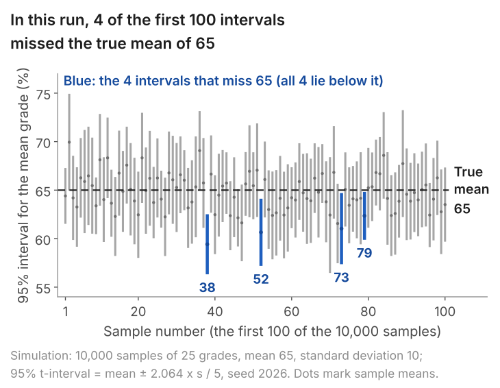
No two intervals are the same. Each sample has its own mean, so each interval sits in a different place, and its own standard deviation, so each has a different length. The line at 65 does not move. In this run 96 of the first 100 intervals cross it and 4 do not. Across all 10,000 samples, 9,518 intervals contain 65: 95.2%.
That is what the 95% describes. It is the success rate of the method: the share of samples in which the interval it produces contains the true mean. It is a statement about the procedure, made before the sample is drawn.
Now go back to the births. We have one interval, 117.63 to 119.77. It is one bar from a picture like Figure 1, and we cannot see the line. Either the population mean is inside this interval or it is not, and nothing about the interval tells us which. What we know is how it was made: by a method whose intervals contain the population mean in about 95% of samples. In everyday use we say the data are compatible with a population mean anywhere between 117.63 and 119.77 ounces.
This is why the sentence "there is a 95% probability that \(\mu\) lies between 117.63 and 119.77" is not right, although it sounds close. Once the interval is computed nothing in that sentence is random: \(\mu\) is a fixed number and so are the two ends. The probability belongs to the method, across repeated samples.
5. Where the multiple comes from, and why 1.96 fails in small samples
The multiple 1.96 is a feature of the normal distribution: it is the point of the standard normal distribution with 2.5% of the probability above it. By symmetry 2.5% lies below -1.96, which leaves 95% between the two.
Suppose first that the data are normally distributed and that we know the population standard deviation \(\sigma\). A sum of independent normal random variables is itself normal (lesson 4), so under random sampling the sample mean is normally distributed in a sample of any size, with standard deviation \(\sigma/\sqrt{n}\). Hence it lies within \(1.96 \times \sigma/\sqrt{n}\) of \(\mu\) in 95% of samples, and the multiple is 1.96 whatever the sample size.
In practice we do not know \(\sigma\), so we use the sample standard deviation \(s\) in its place. In a large sample \(s\) is close to \(\sigma\) and little is lost. In a small sample \(s\) can be well off in either direction: with five grades from our population, where \(\sigma = 10\), \(s\) comes out anywhere between about 4 and 15 in 90% of samples. When \(s\) is low the interval is too short and misses \(\mu\) more often than it should. When \(s\) is high the interval is too long and misses less often, but the gain there is smaller than the loss where \(s\) is low. Across all samples, intervals built with 1.96 succeed less than 95% of the time. To bring the success rate back to 95% the multiple has to be larger than 1.96. The right value comes from the t distribution with \(n - 1\) degrees of freedom (the number of observations, less one for the mean we had to estimate before computing \(s\)):
| Sample size n | 5 | 10 | 25 | 100 | Very large |
|---|---|---|---|---|---|
| Degrees of freedom, n - 1 | 4 | 9 | 24 | 99 | |
| Multiple for a 95% interval | 2.776 | 2.262 | 2.064 | 1.984 | 1.960 |
As the sample grows, \(s\) becomes a better estimate of \(\sigma\), so the multiple falls towards 1.96.
The simulation shows what goes wrong if 1.96 is used anyway. We drew 10,000 samples of each size from the same population of grades and built two intervals from each sample, one with 1.96 and one with the multiple from the table:
| Sample size | Intervals containing 65, using 1.96 | Using the t multiple |
|---|---|---|
| 5 | 88.0% | 94.9% |
| 10 | 91.8% | 95.0% |
| 25 | 94.0% | 95.2% |
With five observations, an interval labelled "95%" that was built with 1.96 contains the true mean in only 88% of samples. With the multiple 2.776 it does what it says. By 25 observations the gap is about a percentage point, and by 100 the two multiples are 1.984 and 1.96 and the choice hardly matters. (The t multiples are exact when the data are normally distributed, as these simulated grades are. For other data in large samples they are a good approximation.) The page on the normal, t, chi-square and F distributions shows how the t distribution is built.
6. An interval by hand
Five workers are paid £10, 12, 13, 16 and 19 an hour (the made-up workers who appear again in lessons 9 to 11). We want a 95% interval for the mean pay in the population they were drawn from.
- Mean. The five figures add to 70, so \(\bar x = 70/5 = 14\).
- Standard deviation. The deviations from the mean are -4, -2, -1, 2 and 5. Their squares, 16, 4, 1, 4 and 25, add to 50. Divide by \(n - 1 = 4\) and take the square root: \(s = \sqrt{50/4} = \sqrt{12.5} = 3.536\).
- Standard error. \(s/\sqrt{n} = 3.536/\sqrt{5} = 1.581\).
- Multiple. With \(n - 1 = 4\) degrees of freedom the table gives 2.776.
- Interval. \(14 \pm 2.776 \times 1.581 = 14 \pm 4.39\), that is, £9.61 to £18.39.
The interval is wide: five workers are compatible with a population mean anywhere from under £10 to over £18. The 95% of the multiple 2.776 rests on pay being normally distributed in the population, which five observations cannot confirm, so the example shows the mechanics. Had we used 1.96 the interval would have been 10.90 to 17.10, which looks more precise and, for normal data, would be right only about 88% of the time.
7. Five real intervals: home advantage in the Premier League
Do home sides score more than away sides? For each of the 380 matches in a Premier League season, take the home side's goals minus the away side's goals. If playing at home made no difference, the population mean of this difference would be zero.
The 380 matches are the whole of a season, so they are not a random sample from a longer list. The population here is the matches that sides like these could play in seasons like it. We treat the season as one draw of 380 matches from that population, and \(\mu\) is the mean difference in it. We also treat the matches as independent of each other, which is an approximation, since each club plays 38 of them. Figure 2 shows the mean and its 95% interval for five seasons.
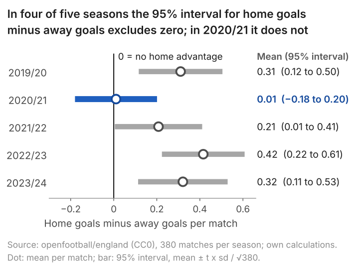
Take 2023/24. The 380 differences have a mean of 0.321 goals and a standard deviation of 2.062, so the standard error is \(2.062/\sqrt{380} = 0.106\). With 379 degrees of freedom the multiple is 1.966, and the interval is \(0.321 \pm 1.966 \times 0.106\), which is 0.113 to 0.529. The data are compatible with a home advantage of anything from about a tenth of a goal to about half a goal a match. Zero is not in the interval.
The table gives the numbers behind two of the five intervals in Figure 2: 2023/24, and 2020/21, the season in which the mean was closest to zero.
| Season | Matches | Mean difference | Std. deviation | Std. error | 95% interval |
|---|---|---|---|---|---|
| 2023/24 | 380 | 0.321 | 2.062 | 0.106 | 0.113 to 0.529 |
| 2020/21 | 380 | 0.011 | 1.889 | 0.097 | -0.180 to 0.201 |
Stata: the code
import delimited "premier-league-matches-2019-24.csv", clear
keep if season == "2023/24"
ttest diff == 0
Stata: what it prints
. ttest diff == 0

One-sample t test
------------------------------------------------------------------------------
Variable |     Obs        Mean    Std. err.   Std. dev.   [95% conf. interval]
---------+--------------------------------------------------------------------
    diff |     380    .3210526    .1057581    2.061605    .1131065    .5289988
------------------------------------------------------------------------------
    mean = mean(diff)                                             t =   3.0357
H0: mean = 0                                     Degrees of freedom =      379

    Ha: mean < 0                 Ha: mean != 0                 Ha: mean > 0
 Pr(T < t) = 0.9987         Pr(|T| > |t|) = 0.0026          Pr(T > t) = 0.0013
R: the code
# Premier League 2023/24: home goals minus away goals (diff) in each of the 380 matches
pl <- read.csv("premier-league-matches-2019-24.csv")
s <- subset(pl, season == "2023/24")
t.test(s$diff, mu = 0)
R: what it prints
> # Premier League 2023/24: home goals minus away goals (diff) in each of the 380 matches
> pl <- read.csv("premier-league-matches-2019-24.csv")
> s <- subset(pl, season == "2023/24")
> t.test(s$diff, mu = 0)

	One Sample t-test

data:  s$diff
t = 3.0357, df = 379, p-value = 0.002565
alternative hypothesis: true mean is not equal to 0
95 percent confidence interval:
 0.1131065 0.5289988
sample estimates:
mean of x
0.3210526
Python: the code
import pandas as pd
from scipy import stats

# Premier League 2023/24: home goals minus away goals (diff) in each of the 380 matches
pl = pd.read_csv("premier-league-matches-2019-24.csv")
s = pl[pl["season"] == "2023/24"]
res = stats.ttest_1samp(s["diff"], popmean=0)
ci = res.confidence_interval(0.95)
print("mean:", s["diff"].mean())
print("standard error:", stats.sem(s["diff"]))
print("t statistic:", res.statistic)
print("degrees of freedom:", res.df)
print("p-value:", res.pvalue)
print("95% interval:", ci.low, ci.high)
Python: what it prints
mean: 0.32105263157894737
standard error: 0.10575810592153756
t statistic: 3.03572599737308
degrees of freedom: 379
p-value: 0.0025653442170994875
95% interval: 0.11310649906992293 0.5289987640879719
The code reads premier-league-matches-2019-24.csv (1,900 matches: season, home, away, home_goals, away_goals, diff). Save it in your working folder first. The same command also reports a t-statistic and a p-value, which are the subject of lessons 7 and 8.
The season 2020/21 stands out. It was played almost entirely behind closed doors because of the pandemic, and the mean difference was 0.011 goals, with an interval from -0.180 to 0.201. That interval contains zero, so the data from that season are compatible with no home advantage at all. Small advantages on either side of zero, such as +0.15 and -0.15, are inside the interval too, so the data do not rule them out. What the interval rules out is an advantage of 0.3 goals or more, the size seen in three of the other four seasons. The interval tells us that the home side's edge was small or absent that season. It does not tell us why.
8. What makes an interval wider or narrower
The margin of error is \(c \times s/\sqrt{n}\), so three things set the width.
- The sample size. The margin is proportional to \(1/\sqrt{n}\), so four times as much data halves it. With the standard deviation of the first 25 births, 22.22, the standard error at \(n = 100\) would be \(22.22/\sqrt{100} = 2.22\), half of 4.444. (The first 100 births give 1.761 because their own standard deviation is smaller, 17.61.) In the birthweight table the standard error falls from 4.44 with 25 births to 0.546 with 1,388.
- The spread of the data. A larger \(s\) means a larger margin. Goal differences have a standard deviation of about 2, which is why 380 matches still leave a margin of 0.2 goals.
- The confidence level. To contain \(\mu\) in a larger share of samples the interval must reach further. For the 1,388 births: 90% gives 117.80 to 119.60 (multiple 1.645), 95% gives 117.63 to 119.77 (1.96) and 99% gives 117.29 to 120.11 (2.576).
The confidence level is our choice, and 95% is a convention. Whichever level is used, state it.
9. Common mistakes
- "There is a 95% probability that the true mean is in this interval." The 95% is the success rate of the method across samples. A computed interval either contains \(\mu\) or does not.
- Reading the interval as a range for individuals. The interval 117.63 to 119.77 is for the mean. Individual birthweights are far more spread out: the mean plus and minus 1.96 standard deviations runs from about 79 to 159 ounces.
- Using the standard deviation where the standard error belongs. \(118.70 \pm 1.96 \times 20.35\) is not a confidence interval for the mean. Divide by \(\sqrt{n}\) first.
- Using 1.96 in a small sample. With five observations the multiple is 2.776, and for normal data intervals built with 1.96 succeed in only about 88% of samples.
- "Zero is in the interval, so the true value is zero." Every value in the interval is compatible with the data. For 2020/21 that includes zero, +0.15 and -0.15.
- "95% of future sample means will fall inside this interval." Future sample means scatter around \(\mu\), not around this sample's mean.
10. Check your understanding
Five questions, marked on the page; every option has an explanation, including the wrong ones. (Without JavaScript the explanations are shown beneath each question.)
1. A sample of 100 workers has a mean hourly wage of £15.00 and a standard deviation of £4.00. Using the multiple 1.984 (99 degrees of freedom), what is the 95% confidence interval for the population mean wage?
15 ± 1.984 × 4 uses the standard deviation of the wages. That range says where individual workers' wages lie. The interval for the mean uses the standard error, 4/√100 = 0.40.
Correct. The standard error is 4/√100 = 0.40, and 15 ± 1.984 × 0.40 = 15 ± 0.79.
This is the mean plus and minus one standard error. An interval that wide contains the population mean in about 68% of samples; 95% needs the multiple 1.984.
4/100 = 0.04 divides the standard deviation by n. The standard error divides by the square root of n: 4/10 = 0.40.
2. In section 4, 10,000 samples of 25 grades gave 10,000 intervals, and 95.2% of them contained the true mean, 65. Suppose the simulation is repeated with samples of 100 grades. What happens to the intervals?
Correct. The multiple is chosen to give a 95% success rate at any sample size. What changes is the standard error, which now estimates 10/√100 = 1 in place of 10/√25 = 2, so the intervals are about half as long.
A larger sample makes each interval shorter. It does not make the method succeed more often: the multiple is chosen so that the success rate is 95% at any sample size.
The length is twice the multiple times s/√n, and √n has doubled. It is the spread of individual grades that stays the same, not the standard error of their mean.
3. A 95% interval for mean birthweight from 25 births is 18 ounces wide. Assuming the standard deviation and the multiple stay the same, how wide is the interval from 100 births?
This divides the width by 4, as if the standard error fell in proportion to n. It falls in proportion to the square root of n, so four times the data halves it.
Correct. Four times the data halves the standard error, and so halves the width. (In the lesson's data the first 100 births give a width of 7.0, because their standard deviation, 17.6, and their multiple, 1.984, are both smaller than for the first 25.)
The width depends on the standard error, s/√n, which shrinks as n grows. It is the spread of individual birthweights that stays the same.
More data make the estimate more precise, not less. Quadrupling n halves the standard error; it does not double it.
4. A sample of 5 workers has a mean of 14 and a standard error of 1.58. Which multiple gives the 95% confidence interval for the population mean? The two-sided 5% values of t are 3.182 with 3 degrees of freedom, 2.776 with 4 and 2.571 with 5.
1.96 is the multiple for large samples. For normal data, intervals built with 1.96 from samples of five contain the true mean in about 88% of samples, not 95%.
2.571 goes with 5 degrees of freedom. For a mean the degrees of freedom are n - 1 = 4, because the five deviations from the sample mean add to zero and only four are free.
Correct. With five observations there are 5 - 1 = 4 degrees of freedom, and 14 ± 2.776 × 1.58 gives 9.6 to 18.4.
3.182 goes with 3 degrees of freedom, which is n - 2: the count for a regression line through five points, where two coefficients are estimated. A mean uses up one, leaving 4.
5. For the 380 Premier League matches of 2020/21, the 95% interval for the mean of home goals minus away goals is -0.18 to 0.20. Which conclusion is justified?
Containing zero means zero is one of the values compatible with the data. So is +0.15, and so is -0.15. The interval does not single out any one of them.
The interval rules a good deal out. An advantage of 0.3 goals a match or more, the size seen in three of the other four seasons, lies outside it.
Correct. Every value from -0.18 to 0.20 is compatible with the data at the 95% level, including zero. Values of 0.3 or more are not.
11. Three questions about intervals
Compute the sample mean and the sample standard deviation. Divide the standard deviation by the square root of the sample size to get the standard error. Multiply the standard error by the t multiple for n - 1 degrees of freedom (1.96 in a large sample), then add the result to the mean and subtract it from the mean.
Use the t table whenever the standard deviation has been estimated from the sample, as it is for every interval in this lesson. The multiple is 2.776 with 5 observations, 2.262 with 10 and 2.064 with 25. It reaches 1.96 only in very large samples, and by 100 observations (1.984) the choice makes little difference.
No. It is a range for the population mean, not for individual observations. For 1,388 birthweights the 95% interval for the mean is 117.6 to 119.8 ounces, while the mean plus and minus 1.96 standard deviations of the data spans roughly 79 to 159 ounces. The interval narrows as the sample grows; the spread of the data does not.
12. Where next
- Lesson 7: hypothesis tests step by step, which asks whether a particular value, such as zero home advantage, is compatible with the data.
- Confidence intervals and t-tests, the explainer: intervals for regression coefficients, one-sided intervals, and why an interval and a two-sided test always agree.
- The normal, t, chi-square and F distributions, for where the multiples come from.
- The course home, which lists all 25 lessons and says which are published.
Stuck on an interval question? Send it
I tutor statistics and econometrics one-to-one, from a first confidence interval through to regression, panel data and time series. Bring the question you are stuck on and we will work through it in the free 30-minute consultation.
Book a free 30-minute consultation Econometrics tutor: how it works
Data and simulation. Birthweights: Wooldridge, Introductory Econometrics: A Modern Approach, data set BWGHT (1,388 births, 1988 National Health Interview Survey); "first 25" and "first 100" are the first rows of the file; results quoted, data not republished. Simulation: grades normal with mean 65 and standard deviation 10; 10,000 samples of each size (5, 10, 25); for each size a fresh numpy default_rng(2026) and rng.normal(65, 10, size=(10000, n)), one row per sample; intervals mean ± multiple × s/√n. Premier League: match results from openfootball/england (CC0), seasons 2019/20 to 2023/24; the file the code reads is premier-league-matches-2019-24.csv. Five-worker example: illustrative data.