
A sample of 25 grades has a mean of 67, an estimate of the population mean; another sample would give another figure. A hypothesis test decides whether a claim about the population mean, here "65 or less", is compatible with the sample, by a rule that rejects a true claim in at most 5% of samples.
In this lesson
1. A claim, a sample, and why 67 does not settle it
Two students disagree about the average grade of economics undergraduates in the UK. Student A claims it is no more than 65%. Student B thinks it is higher. Neither can look up every student's grade, so they agree to draw a random sample of 25 students and see what it says. The sample mean comes out at 67%. (The two students and their numbers are made up for the example. Section 5 uses real data.)
67 is above 65, but a sample mean is not the population mean. Twenty-five different students would have given a different figure, and a sample mean of 67 could turn up even if the population mean were 65. The question a test asks is: how surprising would a sample mean of 67 be if Student A were right?
To answer it we need to know how far a sample mean lies from the population mean, across all the samples of 25 we might have drawn. Lesson 5 showed where the measure comes from. Under random sampling (each grade drawn independently from the same population) the variance of the sample mean around the population mean is the variance of one grade divided by the sample size, \(\sigma^2/n\). Its square root, \(\sigma/\sqrt{n}\), puts it back in marks: it is the standard deviation of the sample mean, called its standard error. Suppose, to keep the first example simple, that individual grades are normally distributed with a known standard deviation of \(\sigma = 10\) marks. Then
$$ \frac{\sigma}{\sqrt{n}} = \frac{10}{\sqrt{25}} = 2 \text{ marks.} $$One grade lies about 10 marks from the population mean, and the mean of 25 grades about 2. Because the grades are normal and drawn independently, their mean is normally distributed too, centred on the population mean.
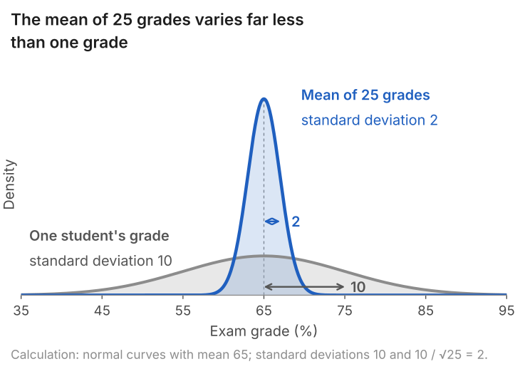
Figure 1 shows the two distributions if the population mean is 65. A single grade of 67 would be unremarkable. A sample mean of 67 is one standard error above 65: further out, but still inside the range that holds 95% of sample means when the population mean is 65. A normal distribution has 95% of its probability within 1.96 standard deviations of its centre, so that range is 65 ± 1.96 × 2, or 61.1 to 68.9. So 67 is weak evidence against Student A.
What students say
“Nicky is an excellent econometrics tutor. He explains complex concepts clearly and makes them much easier to understand.”
“I was completely lost in my economics class, and then I started working Nicky and he totally saved me. He was excellent at explaining the material and extremely accommodating to meet with me many times despite us being in different time zones! Highly recommend working with Nicky!”
“Nicky is a very good and thorough teacher. He has excellent knowledge of econometrics and takes the time to work through your questions. Highly recommended!”
“Really great tutor! Encouraging, knowledgeable, friendly”
“Very good lesson, Nicky is very helpful.”
“Very helpful and clear.”
“I gather it was very useful, thank you!”
“Fantastic!”
2. A test in five steps
Step 1: hypotheses. The claim being tested is called the null hypothesis, H0. What we conclude if the evidence against it is strong enough is the alternative, H1. Student A's claim is the null, and Student B's is the alternative:
$$ H_0: \mu \le 65 \qquad\text{against}\qquad H_1: \mu > 65 . $$Student A's claim covers many values of \(\mu\): 65, 64, 60 and so on. We test it at its boundary, \(\mu = 65\). Of all the values the claim allows, 65 is the one under which a high sample mean is least surprising. If the sample is hard to square with 65, it is harder still to square with 64 or 60.
Step 2: test statistic. We measure how far the sample mean is from 65 in standard errors:
$$ z = \frac{\bar x - 65}{\sigma/\sqrt{n}} = \frac{\bar x - 65}{2} . $$In words: z = (sample mean minus the hypothesised mean) divided by the standard error.
If the population mean is 65, the sample mean is normal with mean 65 and standard error 2 (section 1). Subtracting the mean of a normal variable and dividing by its standard deviation gives a normal variable with mean 0 and standard deviation 1 (lesson 2 on standardising). Hence \(Z = (\bar X - 65)/2\) follows the standard normal distribution, with 95% of its values between -1.96 and 1.96, and the \(z\) we compute from our sample is one draw from it. (As in lesson 6, a capital letter marks a quantity that varies from sample to sample and the lower-case letter the value our sample gives: \(\bar X\) and \(\bar x\), \(Z\) and \(z\).) A large positive \(z\) is what we would expect to see if Student B were right.
Step 3: significance level and rejection region. We will reject H0 when \(z\) is too large to be believable under H0. "Too large" needs a cut-off, and wherever we put it there is some chance that a true H0 produces a \(z\) beyond it. The significance level is the largest chance of rejecting a true H0 that we are prepared to accept. We use 5%, the conventional choice; lesson 8 shows what changes at 1%. The standard normal distribution has 5% of its area above 1.645, so the rule is: reject H0 if \(z > 1.645\). The values of the statistic that lead to rejection are the rejection region, and the cut-off, 1.645, is called the critical value. On the scale of the sample mean the same cut-off is \(65 + 1.645 \times 2 = 68.29\).
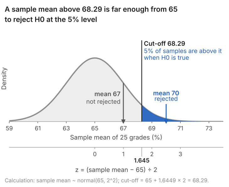
Everything up to here was settled without a single grade collected: the cut-off 68.29 is the same whatever sample arrives. Fixing it first stops us from moving it to suit the sample, and it gives the rule a known error rate. In lesson 8 we draw 10,000 samples from a population whose mean is 65, and 498 of them, 5.0%, have a sample mean above 68.29.
Step 4: compute. The sample mean is 67, so \(z = (67 - 65)/2 = 1.00\).
Step 5: decide. 1.00 is below 1.645, so we do not reject H0. In words: at the 5% level, a sample mean of 67 from 25 students is compatible with a population mean of 65 or less.
Had the sample mean been 70, \(z\) would have been \((70 - 65)/2 = 2.5\), which is above 1.645. We would reject H0 and conclude that the population mean is above 65.
"Do not reject" is not "accept". A sample mean of 67 is compatible with \(\mu = 65\). It is also compatible with 66, 67 or 68: the same test, run with any value above 63.7 in place of 65, would not reject H0 either (63.7 is \(67 - 1.645 \times 2\)). The test has not shown that Student A is right. It has shown that this sample cannot tell the two students apart.
Recap: the five steps of a hypothesis test
- State the hypotheses. The null, H0, is the claim being tested; the alternative, H1, is what we conclude if the evidence against H0 is strong enough. Both are statements about the population.
- Choose a test statistic and find how it is distributed if H0 is true.
- Choose the significance level and find the critical value, which fixes the rejection region.
- Compute the statistic from the sample.
- Decide, and say what the decision means in words.
Remarks. The population mean \(\mu\) is fixed and unknown. The sample mean is random until the sample is drawn, and we write it \(\bar X\) while it is; once the sample is in hand it is a number, \(\bar x\) (67 here). Steps 1 to 3 are done before the data are seen; only steps 4 and 5 use the sample.
3. One tail or two
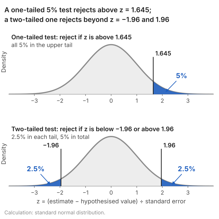
Student B's alternative pointed in one direction, \(\mu > 65\), so only a high sample mean counted against H0 and all 5% of the rejection region went in the upper tail. That is a one-tailed (or one-sided) test.
Suppose a third student claims the population mean is exactly 65, and we have no view about whether it is higher or lower:
$$ H_0: \mu = 65 \qquad\text{against}\qquad H_1: \mu \ne 65 . $$Now a sample mean far below 65 counts against H0 as much as one far above it. The 5% is split between the two tails, 2.5% in each, and the rule becomes: reject H0 if \(z\) is above 1.96 or below -1.96. This is a two-tailed test.
| Sample mean | z | One-tailed test (cut-off 1.645) | Two-tailed test (cut-off ±1.96) |
|---|---|---|---|
| 67 | 1.00 | Do not reject | Do not reject |
| 68.5 | 1.75 | Reject | Do not reject |
| 70 | 2.50 | Reject | Reject |
The table applies both tests to three possible sample means. For 67 and for 70 the two tests agree. For 68.5 they do not: \(z = 1.75\) is beyond the one-tailed cut-off and inside the two-tailed one. So the choice between one tail and two can change the conclusion, and it has to be made at step 1, from the question being asked. Choosing the tail after seeing which way the sample points means rejecting whenever \(z\) is beyond 1.645 in either direction, which happens in 10% of samples when H0 is true. The test would then be a 10% test reported as a 5% one.
4. When the standard deviation is estimated: the t-test
So far we have assumed that the standard deviation of grades, \(\sigma = 10\), is known. With real data it is not, and we estimate it from the same sample. Here are the grades of nine students (made-up numbers, chosen so that the arithmetic is short):
58, 62, 66, 66, 68, 70, 70, 74, 78.
- Mean. The nine grades add to 612, so \(\bar x = 612/9 = 68\).
- Standard deviation. The deviations from 68 are -10, -6, -2, -2, 0, 2, 2, 6 and 10. Their squares, 100, 36, 4, 4, 0, 4, 4, 36 and 100, add to 288. Divide by \(n - 1 = 8\) and take the square root: \(s = \sqrt{288/8} = \sqrt{36} = 6\).
- Standard error. \(s/\sqrt{n} = 6/\sqrt{9} = 2\).
- Test statistic. The same formula as before, with \(s\) in place of \(\sigma\): \(t = (68 - 65)/2 = 1.5\).
The cut-off is no longer 1.645, because \(s\) is itself an estimate, and from nine observations a rough one. If grades were normal with a true standard deviation of 6, another nine students would give an \(s\) anywhere from about 3.5 to 8.4 in 90% of samples, so the standard error would range from about 1.2 to 2.8. The statistic now has a denominator that changes from sample to sample as well as a numerator, so it varies more than \(Z\) does. Samples in which \(s\) comes out low give a statistic that is too far from zero, and they add more to the area beyond 1.645 than samples with a high \(s\) take away. Used with 1.645, the test would reject a true H0 in more than 5% of samples when the mean is exactly 65.
If the grades are normally distributed and the population mean is 65, the statistic, written \(T = (\bar X - 65)/(s/\sqrt{n})\) with \(s\) treated as random, follows the t distribution with \(n - 1 = 8\) degrees of freedom. The count is \(n - 1\) because \(s\) is built from the deviations about the sample mean, and those nine deviations must add to zero, so only eight of them are free (lesson 3 explains why the variance divides by \(n - 1\)). The t distribution with 8 degrees of freedom has 5% of its area above 1.860, so the rule "reject when \(t > 1.860\)" rejects a true H0 in at most 5% of samples, and in 5% when the mean is exactly 65. The test is called a t-test after this distribution. Here \(t = 1.5\), below 1.860, so we do not reject H0: nine students with a mean of 68 are compatible with a population mean of 65 or less.
The table puts the test on one line, as software reports it: the sample size, the three numbers worked out above, the statistic, its degrees of freedom and the critical value it is compared with.
| n | Mean | Std. deviation | Std. error | t | Degrees of freedom | 5% cut-off, one-tailed |
|---|---|---|---|---|---|---|
| 9 | 68 | 6 | 2 | 1.5 | 8 | 1.860 |
Stata: the code
clear
input grade
58
62
66
66
68
70
70
74
78
end
ttest grade == 65
Stata: what it prints
. ttest grade == 65

One-sample t test
------------------------------------------------------------------------------
Variable |     Obs        Mean    Std. err.   Std. dev.   [95% conf. interval]
---------+--------------------------------------------------------------------
   grade |       9          68           2           6    63.38799    72.61201
------------------------------------------------------------------------------
    mean = mean(grade)                                            t =   1.5000
H0: mean = 65                                    Degrees of freedom =        8

    Ha: mean < 65               Ha: mean != 65                 Ha: mean > 65
 Pr(T < t) = 0.9140         Pr(|T| > |t|) = 0.1720          Pr(T > t) = 0.0860
R: the code
# nine grades: test H0: mean = 65 against Ha: mean > 65, then the two-sided version with the 95% interval
grades <- c(58, 62, 66, 66, 68, 70, 70, 74, 78)
t.test(grades, mu = 65, alternative = "greater")
t.test(grades, mu = 65)
R: what it prints
> # nine grades: test H0: mean = 65 against Ha: mean > 65, then the two-sided version with the 95% interval
> grades <- c(58, 62, 66, 66, 68, 70, 70, 74, 78)
> t.test(grades, mu = 65, alternative = "greater")

	One Sample t-test

data:  grades
t = 1.5, df = 8, p-value = 0.086
alternative hypothesis: true mean is greater than 65
95 percent confidence interval:
 64.2809     Inf
sample estimates:
mean of x
       68

> t.test(grades, mu = 65)

	One Sample t-test

data:  grades
t = 1.5, df = 8, p-value = 0.172
alternative hypothesis: true mean is not equal to 65
95 percent confidence interval:
 63.38799 72.61201
sample estimates:
mean of x
       68
Python: the code
from scipy import stats

# nine grades: test H0: mean = 65 against Ha: mean > 65, then the two-sided version with the 95% interval
grades = [58, 62, 66, 66, 68, 70, 70, 74, 78]
res = stats.ttest_1samp(grades, popmean=65, alternative="greater")
print("t statistic:", res.statistic)
print("degrees of freedom:", res.df)
print("one-sided p-value:", res.pvalue)

res2 = stats.ttest_1samp(grades, popmean=65)
ci = res2.confidence_interval(0.95)
print("two-sided p-value:", res2.pvalue)
print("95% interval:", ci.low, ci.high)
Python: what it prints
t statistic: 1.5
degrees of freedom: 8
one-sided p-value: 0.08600164597595561
two-sided p-value: 0.17200329195191122
95% interval: 63.38799172959167 72.61200827040832
Each program also prints p-values, which are the subject of lesson 8, and a confidence interval.
The cut-off depends on the sample size. As the sample grows, \(s\) settles on \(\sigma\) (the law of large numbers), the extra variation from estimating \(\sigma\) dies away, and the cut-off falls towards the normal values, 1.645 (one-tailed) and 1.96 (two-tailed). With few observations it is well above them:
| Degrees of freedom | 4 | 8 | 24 | 99 | Very large |
|---|---|---|---|---|---|
| 5% cut-off, one-tailed | 2.132 | 1.860 | 1.711 | 1.660 | 1.645 |
| 5% cut-off, two-tailed | 2.776 | 2.306 | 2.064 | 1.984 | 1.960 |
The two-tailed critical values are the multiples used for 95% confidence intervals in lesson 6: the multiple in an interval and the cut-off in a test are the same number. (The t cut-offs are exact when the data are normally distributed. For other data they are a good approximation in large samples, provided the observations are drawn independently and have a finite variance: the central limit theorem then makes the sample mean approximately normal, and \(s\) is close to \(\sigma\).)
5. A real test: is there home advantage?
For each of the 380 matches of a Premier League season, take the home side's goals minus the away side's goals. If playing at home made no difference, the population mean of this difference would be zero. (As in lesson 6, the 380 matches are the whole season, not a random sample from a longer list. The population is the matches that sides like these could play in seasons like it, and the 380 matches are treated as independent draws from it, which is an approximation, since each club plays 38 of them.) Before looking at the data we allow that the difference could go either way, so the test is two-tailed.
- Hypotheses. \(H_0: \mu = 0\) against \(H_1: \mu \ne 0\), where \(\mu\) is the mean of home goals minus away goals.
- Test statistic. \(t = \bar x / (s/\sqrt{n})\), the mean difference in standard errors from zero. Goal differences are whole numbers, so they are not normal and the t distribution is not exact here. With 380 matches it is a close approximation: treating the matches as independent draws with a finite variance, the central limit theorem makes the sample mean approximately normal, and \(s\) is close to \(\sigma\). Hence, if H0 is true, \(T = \bar X/(s/\sqrt{n})\) has approximately a t distribution with \(n - 1 = 379\) degrees of freedom.
- Level and rejection region. At the 5% level, reject if \(t\) is above 1.966 or below -1.966.
- Compute. For 2023/24, \(t = 3.04\). For 2020/21, \(t = 0.11\). The table shows the working.
- Decide. 3.04 is above 1.966, so we reject H0 for 2023/24. 0.11 is not, so we do not reject H0 for 2020/21.
| Season | Matches | Mean difference | Std. deviation | Std. error | t | Decision at 5% |
|---|---|---|---|---|---|---|
| 2023/24 | 380 | 0.321 | 2.062 | 0.106 | 3.04 | Reject H0 |
| 2020/21 | 380 | 0.011 | 1.889 | 0.097 | 0.11 | Do not reject H0 |
Each row is one season: the mean of the 380 differences, their standard deviation, the standard error (the standard deviation divided by \(\sqrt{380}\)) and the t-statistic (the mean divided by the standard error). For 2023/24, \(0.321/0.106 = 3.03\); the software, working with unrounded figures, prints 3.04.
Stata: the code
import delimited "premier-league-matches-2019-24.csv", clear
keep if season == "2023/24"
ttest diff == 0
Stata: what it prints
. ttest diff == 0

One-sample t test
------------------------------------------------------------------------------
Variable |     Obs        Mean    Std. err.   Std. dev.   [95% conf. interval]
---------+--------------------------------------------------------------------
    diff |     380    .3210526    .1057581    2.061605    .1131065    .5289988
------------------------------------------------------------------------------
    mean = mean(diff)                                             t =   3.0357
H0: mean = 0                                     Degrees of freedom =      379

    Ha: mean < 0                 Ha: mean != 0                 Ha: mean > 0
 Pr(T < t) = 0.9987         Pr(|T| > |t|) = 0.0026          Pr(T > t) = 0.0013
R: the code
# Premier League 2023/24: home goals minus away goals (diff) in each of the 380 matches
pl <- read.csv("premier-league-matches-2019-24.csv")
s <- subset(pl, season == "2023/24")
t.test(s$diff, mu = 0)
R: what it prints
> # Premier League 2023/24: home goals minus away goals (diff) in each of the 380 matches
> pl <- read.csv("premier-league-matches-2019-24.csv")
> s <- subset(pl, season == "2023/24")
> t.test(s$diff, mu = 0)

	One Sample t-test

data:  s$diff
t = 3.0357, df = 379, p-value = 0.002565
alternative hypothesis: true mean is not equal to 0
95 percent confidence interval:
 0.1131065 0.5289988
sample estimates:
mean of x
0.3210526
Python: the code
import pandas as pd
from scipy import stats

# Premier League 2023/24: home goals minus away goals (diff) in each of the 380 matches
pl = pd.read_csv("premier-league-matches-2019-24.csv")
s = pl[pl["season"] == "2023/24"]
res = stats.ttest_1samp(s["diff"], popmean=0)
ci = res.confidence_interval(0.95)
print("mean:", s["diff"].mean())
print("standard error:", stats.sem(s["diff"]))
print("t statistic:", res.statistic)
print("degrees of freedom:", res.df)
print("p-value:", res.pvalue)
print("95% interval:", ci.low, ci.high)
Python: what it prints
mean: 0.32105263157894737
standard error: 0.10575810592153756
t statistic: 3.03572599737308
degrees of freedom: 379
p-value: 0.0025653442170994875
95% interval: 0.11310649906992293 0.5289987640879719
The code reads premier-league-matches-2019-24.csv (1,900 matches: season, home, away, home_goals, away_goals, diff). Save it in your working folder first. Change the season in the code to "2020/21" for the second row.
2023/24. The mean difference is three standard errors above zero, far beyond 1.966. We reject H0 at the 5% level: if there were no home advantage, a mean difference three standard errors or more from zero would occur in fewer than 5% of seasons.
2020/21. The mean difference is 0.011 goals, about a tenth of a standard error from zero. We do not reject H0. That season was played almost entirely behind closed doors because of the pandemic, and in it the home side's advantage cannot be told apart from zero.
The second result needs the same care as the grades. First, "do not reject" again does not mean "zero": the 95% interval for 2020/21 runs from -0.18 to 0.20 goals a match, so a small advantage in either direction, such as +0.15 or -0.15, is not ruled out either. Second, the test compares one season with a benchmark of zero. It does not show that the absence of crowds was the cause. That would need an argument about what else differed that season.
6. Common mistakes
- Writing hypotheses about the sample. "H0: \(\bar x = 65\)" is not a hypothesis. We can see \(\bar x\). The hypotheses are about the population mean \(\mu\), which we cannot see.
- "Accepting" the null. A sample mean of 67 did not reject \(\mu \le 65\), and it would not have rejected \(\mu = 68\) either. Write "do not reject", and say what the data are compatible with.
- Choosing the tail after seeing the data. With \(z = 1.75\) the one-tailed test rejects and the two-tailed one does not. Decide which test the question calls for at step 1.
- Using 1.645 or 1.96 with a small sample and an estimated standard deviation. With nine observations the one-tailed cut-off is 1.860.
- Dividing by the standard deviation. The statistic is the distance from the hypothesised value in standard errors, \(s/\sqrt{n}\), not in standard deviations.
- Leaving out the level. "We reject H0" is incomplete. "We reject H0 at the 5% level" says how strict the test was.
7. Check your understanding
Five questions, marked on the page; every option has an explanation, including the wrong ones. (Without JavaScript the explanations are shown beneath each question.)
1. A lecturer says the mean mark on her module is 60. A student suspects it is lower and takes a random sample of 36 marks. Which pair of hypotheses fits the student's test?
Correct. The null is the claim being tested, stated as a value of the population mean. The alternative is what the student suspects, and it sets the direction of the test.
The two are the wrong way round. The null is the claim being tested, and the test works at its boundary value (60 here), so that we can work out how sample means would behave if it were true.
Hypotheses are statements about the population. The sample mean is a number we compute from the sample and can read off; there is nothing to test about it.
2. Grades have a known standard deviation of 12. A sample of 36 students has a mean of 63. For H0: μ ≤ 60 against H1: μ > 60, what is the z-statistic?
(63 - 60)/12 divides by the standard deviation of individual grades. The sample mean varies much less than one grade: its standard error is 12/√36 = 2.
Correct. The standard error is 12/√36 = 2, and z = (63 - 60)/2 = 1.5: the sample mean is one and a half standard errors above 60.
1.645 is the critical value that z is compared with in a one-sided 5% test. It is not computed from the sample.
(63 - 60)/(12/36) divides the standard deviation by n. The standard error divides by the square root of n: 12/6 = 2.
3. For H0: μ ≤ 65 against H1: μ > 65 at the 5% level, the critical value is 1.645 and the sample gives z = 1.00. Which conclusion does the evidence support?
The sample does not show that. A z of 1.00 puts the sample mean one standard error above 65, which is what we would expect to see if the true mean were one standard error above 65.
A sample mean above 65 is not enough. Sample means vary, and one this far above 65 turns up in about 16% of samples when the true mean is 65.
Correct. z = 1.00 is below 1.645, so the data are not surprising enough to reject the null. That is a statement about the evidence, not proof that the null is true.
4. A sample gives z = 1.75. The one-sided 5% critical value is 1.645 and the two-sided one is 1.96. A researcher who had no view about the direction beforehand sees the positive z and reports a one-sided test. What is the problem?
Correct. Choosing the tail after seeing the sign means rejecting whenever z is beyond 1.645 in either direction, which happens in 10% of samples when the null is true.
Whether to use z or t depends on whether the standard deviation is known, not on the number of tails. The problem here is when the tail was chosen.
It is above the one-sided cut-off and below the two-sided one, so the conclusion depends on the choice. That is why the choice has to be made before the data are seen.
5. Nine students have a mean grade of 68 and a sample standard deviation of 6, so t = (68 - 65)/2 = 1.5. Which critical value should a one-sided 5% test use?
1.645 is right when the standard deviation is known, or the sample is large. Here it is estimated from nine observations, so the t distribution is needed.
Correct. The standard deviation is computed from deviations about the sample mean, which uses one degree of freedom: 9 - 1 = 8. Since 1.5 is below 1.860, the null is not rejected.
The degrees of freedom are n - 1, not n, because the nine deviations from the sample mean add to zero and only eight are free.
8. Three questions about tests
State the null and alternative hypotheses about the population. Choose a test statistic and find its distribution if the null is true. Choose a significance level and the rejection region. Compute the statistic from the sample. Reject the null if the statistic falls in the rejection region, and state the conclusion in words, with the level.
Because a sample that is compatible with the null is compatible with other values too. A sample mean of 67 with a standard error of 2 does not reject a population mean of 65, and would not reject 66, 67 or 68 either. The data have failed to rule the null out; they have not shown it to be true.
From the question, before seeing the data. If only a difference in one direction would count against the null (the mean is above 65, say), use a one-tailed test. If a difference in either direction would count, use a two-tailed test. If the question gives no direction, use two tails, which is also what regression software reports.
9. Where next
- Lesson 8: p-values, Type I and II errors, power: how strong the evidence is, and how often a test gets the decision wrong.
- Hypothesis testing explained, the explainer: the same example taken further, and how the logic carries over to regression coefficients.
- The normal, t, chi-square and F distributions, for where the cut-offs come from.
- Lesson 6: confidence intervals (previous) and the course home, which lists all 25 lessons and says which are published.
Not sure which test a question wants? Send it
I tutor statistics and econometrics one-to-one, from a first hypothesis test through to regression, panel data and time series. Bring the question you are stuck on and we will work through it in the free 30-minute consultation.
Book a free 30-minute consultation Econometrics tutor: how it works
Data. Grade examples: illustrative numbers (a normal population with standard deviation 10; nine made-up grades). Premier League: match results from openfootball/england (CC0), seasons 2020/21 and 2023/24, 380 matches each; the file the code reads is premier-league-matches-2019-24.csv.