
The probability distribution of a discrete random variable lists every value it can take, with its probability: for home goals, ten values and ten probabilities. A few numbers summarise it, and samples estimate them: the expectation, a probability-weighted average; the variance and standard deviation, its spread; and, for two variables, the covariance and correlation, how they move together.
In this lesson
- The centre of a distribution: expectation
- How far values lie from the centre: variance and standard deviation
- Changing units: the rules for means and variances
- Do two variables move together? Covariance
- Correlation, and why zero correlation is not independence
- The variance of a sum
- From the distribution to data, and why n - 1
- Common mistakes
- Check your understanding: five marked questions
- Three questions about variance and correlation
- Where next
1. The centre of a distribution: expectation
How many goals does a home side score in a match, on average? Lesson 2 set out the distribution of home goals in the 1,900 Premier League matches of 2019/20 to 2023/24. Draw one of those matches at random and let \(X\) be the home side's goals: as in lesson 2, the capital \(X\) is the random variable and the lower-case \(x\) a value it takes. Then \(P(X = x)\) is the share of the 1,900 matches with \(x\) home goals: \(P(X = 1) = 609/1{,}900 = 0.321\). We want one number for where this distribution is centred.
The expectation weights each value by its probability and adds up:
$$ E[X] = \sum_x x\, P(X = x) . $$In words: expectation = the sum, over every value, of the value times its probability.
Draw a match at random again and again, putting it back each time. By the law of large numbers of lesson 4, the share of draws with each value settles at its probability. Hence the average of the goals drawn, each value times its share, settles at \(E[X]\): the expectation is the long-run average.
Each probability here is a number of matches over 1,900, so the sum can be done in whole numbers, with no rounding: multiply each value by its matches, add, and divide by 1,900.
| Home goals \(x\) | Matches | \(x\) × matches |
|---|---|---|
| 0 | 438 | 0 |
| 1 | 609 | 609 |
| 2 | 448 | 896 |
| 3 | 245 | 735 |
| 4 | 100 | 400 |
| 5 | 42 | 210 |
| 6 | 11 | 66 |
| 7 | 4 | 28 |
| 8 | 1 | 8 |
| 9 | 2 | 18 |
| Total | 1,900 | 2,970 |
The expectation need not be a value \(X\) can take: no home side scores 1.563 goals.
A 0/1 variable turns a share into a mean, which lessons 4 and 5 use. Let \(W = 1\) if the home side wins and \(W = 0\) otherwise, with \(P(W = 1) = p\). Then
$$ E[W] = 0 \times (1 - p) + 1 \times p = p . $$The mean of a 0/1 variable is the probability of a 1. The home side won 838 of the 1,900 matches, so the mean of \(W\) is the share of home wins, 0.441. For a continuous variable, such as a birthweight, a density replaces the probabilities and an integral replaces the sum; the meaning is unchanged.
We write \(\mu\) for \(E[X]\), or \(\mu_X\) when two variables must be told apart; expectation, expected value and population mean are three names for it. Books also write \(\mathbb{E}(X)\); the choice of letters is cosmetic. The population mean is a fixed feature of the distribution: 1.563 here. A sample mean is computed from data and changes from sample to sample: five samples of 10 matches drawn at random from the 1,900 gave 2.0, 2.2, 1.3, 1.0 and 1.1 goals (lesson 4 studies this variation).
The same weighting gives the expectation of any function \(g\) of \(X\):
$$ E[g(X)] = \sum_x g(x)\, P(X = x) . $$In words: the average in the population of g(X). The variance below is the choice \(g(x) = (x - \mu)^2\); the covariance in section 4 weights a function of two variables by their joint probabilities.
What students say
“Nicky is an excellent econometrics tutor. He explains complex concepts clearly and makes them much easier to understand.”
“I was completely lost in my economics class, and then I started working Nicky and he totally saved me. He was excellent at explaining the material and extremely accommodating to meet with me many times despite us being in different time zones! Highly recommend working with Nicky!”
“Nicky is a very good and thorough teacher. He has excellent knowledge of econometrics and takes the time to work through your questions. Highly recommended!”
“Really great tutor! Encouraging, knowledgeable, friendly”
“Very good lesson, Nicky is very helpful.”
“Very helpful and clear.”
“I gather it was very useful, thank you!”
“Fantastic!”
2. How far values lie from the centre: variance and standard deviation
The mean gives the centre of the distribution and does not measure how far the values lie from it. A mean of 1.563 goals does not show whether scores of 0 or 5 are rare or routine: a side that scored 1 goal in 44% of its matches and 2 in the rest would also average 1.56. Our home sides scored none in 23% of matches and 5 or more in 3%. We need a number for the spread.
A first idea is the average deviation from the mean, where a deviation \(x - \mu\) is how far a value lies above the mean. The probabilities add to 1 and \(\sum_x x\,P(X = x) = \mu\), so for every distribution
$$ \begin{aligned} E[X - \mu] &= \sum_x (x - \mu)\, P(X = x) \\ &= \mu - \mu = 0 . \end{aligned} $$Deviations above the mean cancel those below it, so their average says nothing about spread. We square them before averaging instead. A square is never negative, so nothing cancels, and a value twice as far from the mean counts four times as much. Distances without their signs, \(|x - \mu|\), would also stop the cancelling, but squares obey a rule that they do not: the variance of a sum follows from the two variances and the covariance (section 6), and under random sampling that rule gives the variance of the mean of \(n\) observations, \(\sigma^2/n\). The variance is the average squared distance from the mean, the choice \(g(x) = (x - \mu)^2\):
$$ \begin{aligned} \sigma^2 = \operatorname{Var}(X) &= E[(X - \mu)^2] \\ &= \sum_x (x - \mu)^2\, P(X = x) . \end{aligned} $$In words: variance = the probability-weighted average of the squared distances from the mean.
The table works it out for home goals, with deviations from the unrounded mean, 2,970/1,900, and each probability as matches/1,900.
| Home goals \(x\) | Matches | Deviation \(x - \mu\) | \((x - \mu)^2\) × matches/1,900 |
|---|---|---|---|
| 0 | 438 | -1.563 | 0.563 |
| 1 | 609 | -0.563 | 0.102 |
| 2 | 448 | 0.437 | 0.045 |
| 3 | 245 | 1.437 | 0.266 |
| 4 | 100 | 2.437 | 0.313 |
| 5 | 42 | 3.437 | 0.261 |
| 6 | 11 | 4.437 | 0.114 |
| 7 | 4 | 5.437 | 0.062 |
| 8 | 1 | 6.437 | 0.022 |
| 9 | 2 | 7.437 | 0.058 |
| Total | 1,900 | 1.806 |
The terms add to \(\operatorname{Var}(X) = 1.806\), in goals squared, since each is a squared number of goals.
The standard deviation
The square root returns the variance to goals, the units the data are measured in, and gives the standard deviation:
$$ \sigma = \sqrt{\operatorname{Var}(X)} = \sqrt{1.806} = 1.344 \text{ goals.} $$In words: standard deviation = square root of the variance.
It reads as a typical distance from the mean, but "typical" needs care: it is the square root of the average squared distance, not the average distance. The average distance, \(E[\,|X - \mu|\,]\), called the mean absolute deviation, is 1.082 goals. Squaring gives large distances more weight, so the standard deviation is the larger; both are in goals and on the same scale.
A shortcut avoids the deviations:
$$ \operatorname{Var}(X) = E[X^2] - \mu^2 . $$In words: variance = the mean of the squares minus the square of the mean.
Show where the shortcut comes from
- Expand the square. \((x - \mu)^2 = x^2 - 2\mu x + \mu^2\).
- Weight by the probabilities and add, term by term. The first term gives \(E[X^2]\), the second \(-2\mu \sum_x x\,P(X = x) = -2\mu^2\), and the third \(\mu^2\), since the probabilities add to 1.
- Add the three. $$ \begin{aligned} & E[X^2] - 2\mu^2 + \mu^2 \\ &= E[X^2] - \mu^2 . \end{aligned} $$
For home goals the squared values times their matches add to 8,074, so \(E[X^2] = 8{,}074/1{,}900 = 4.2495\) and
$$ \begin{aligned} \operatorname{Var}(X) &= 4.2495 - \left(\tfrac{2970}{1900}\right)^2 \\ &= 4.2495 - 2.4435 = 1.8060 . \end{aligned} $$For a 0/1 variable, \(W^2 = W\) (as \(0^2 = 0\) and \(1^2 = 1\)), so \(E[W^2] = p\) and
$$ \operatorname{Var}(W) = p - p^2 = p(1 - p) , $$which is \(0.441 \times 0.559 = 0.2465\) for home wins. It is largest, 0.25, at \(p = 0.5\), where the outcome is least predictable: a guess is wrong half the time.
Definition: expectation, variance and standard deviation
For a discrete random variable \(X\):
$$ \begin{aligned} \mu = E[X] &= \sum_x x\, P(X = x) , \\ \sigma^2 = \operatorname{Var}(X) &= E[(X - \mu)^2] , \\ \sigma &= \sqrt{\operatorname{Var}(X)} . \end{aligned} $$Remarks. The expectation is the probability-weighted average of the values, the variance the probability-weighted average of the squared distances from it, and the standard deviation the square root of the variance, back in the units of the data. All three are fixed features of the distribution, not numbers computed from a sample. The standard deviation is not the average distance from the mean: for home goals the two are 1.344 and 1.082.
3. Changing units: the rules for means and variances
The same quantity can be recorded in different units, ounces or grams, dollars or cents, and its mean and variance change with the units by fixed rules. A change of units or of the zero point turns \(X\) into \(a + bX\): a weight in grams is the weight in ounces times 28.3495, so \(a = 0\) and \(b = 28.3495\). Weighting \(a + bx\) by the probabilities and adding gives \(a\), as the probabilities add to 1, plus \(b\mu\):
$$ E[a + bX] = a + b\,E[X] . $$In words: shift and rescale the variable, and its mean is shifted and rescaled in the same way.
Each deviation becomes \((a + bx) - (a + b\mu) = b(x - \mu)\): the shift cancels and the deviation is multiplied by \(b\). So every squared deviation, and their average, is multiplied by \(b^2\):
$$ \operatorname{Var}(a + bX) = b^2 \operatorname{Var}(X) . $$In words: adding a constant leaves the variance alone; multiplying by b multiplies the variance by b squared and the standard deviation by |b|.
The rules hold for the mean and standard deviation of data too, since the values and their mean move together. The 1,388 birthweights of lesson 6, a sample of births, have a mean of 118.70 ounces and a standard deviation of 20.35 ounces. In grams these are \(118.70 \times 28.3495 = 3{,}365\) and \(20.35 \times 28.3495 = 577\), and the variance is \(28.3495^2 = 803.7\) times its value in ounces squared.
For two random variables, the expectation of a sum is the sum of the expectations, the additive property of expectations:
$$ E[X + Y] = E[X] + E[Y] . $$In words: the mean of a sum = the sum of the means.
Show why the mean of a sum is the sum of the means
Weight \(x + y\) by the joint probabilities and add. Summing the joint probabilities over the other variable gives the marginal ones, so the \(x\) parts add up to \(E[X]\) and the \(y\) parts to \(E[Y]\).
No step of the derivation uses how \(X\) and \(Y\) are related, so the rule holds whether or not they are: total goals average \(1.563 + 1.310 = 2.873\) a match. It extends to any number of variables; lesson 4 uses it for the sample mean. The variance of a sum is not this simple: it depends on whether the variables move together.
4. Do two variables move together? Covariance
Economics asks whether two variables move together: whether pay is higher for workers with more education, or birthweight lower when the mother smoked. The covariance is one number for this: the expectation of the product of the two deviations from their means, each pair of values weighted by its joint probability:
$$ \operatorname{Cov}(X, Y) = E[(X - \mu_X)(Y - \mu_Y)] . $$In words: covariance = the probability-weighted average of the product of the two deviations from their means.
The product is positive when both variables are above their means or both below, and negative when one is above and the other below. So the covariance is positive when the variables move together and negative when they move in opposite directions. Lesson 9 draws this as four quadrants around the point of means.
Take the table of two 0/1 variables from lesson 2. Their means are their probabilities of a 1, \(\mu_X = 0.3\) and \(\mu_Y = 0.5\), and each pair of values contributes its product of deviations times its joint probability:
| \(x\), \(y\) | Joint probability | \((x - 0.3)(y - 0.5)\) | Product × probability |
|---|---|---|---|
| 0, 0 | 0.4 | 0.15 | 0.06 |
| 1, 0 | 0.1 | -0.35 | -0.035 |
| 0, 1 | 0.3 | -0.15 | -0.045 |
| 1, 1 | 0.2 | 0.35 | 0.07 |
| Total | 1 | 0.05 |
The two pairs in which \(X\) and \(Y\) are equal have positive products and contribute \(0.06 + 0.07 = 0.13\); the two in which they differ contribute \(-0.035 - 0.045 = -0.08\). The positive part is the larger, so the covariance is positive. Expanding the product, as for the variance shortcut, gives
$$ \operatorname{Cov}(X, Y) = E[XY] - \mu_X\,\mu_Y . $$In words: covariance = the mean of the product minus the product of the means.
Here \(XY = 1\) only when both are 1, so \(E[XY] = 0.2\), and \(0.2 - 0.3 \times 0.5 = 0.05\): the same answer.
A covariance is in the units of one variable times those of the other, since each product multiplies the two deviations. For the 526 US workers of the WAGE1 data (1976), the covariance of the hourly wage and years of education, computed from the data as in section 7, is 4.151 dollars an hour times years. Its size cannot be read on its own, since it changes with the units: with the wage in cents every wage deviation is 100 times larger, and the same workers give 415.1. A variable's covariance with itself is its variance: put \(Y = X\) in the definitions to convince yourself.
5. Correlation: covariance without units
To measure how closely two variables move together on a scale free of their units, divide the covariance by both standard deviations:
$$ \operatorname{Corr}(X, Y) = \rho = \frac{\operatorname{Cov}(X, Y)}{\sigma_X\, \sigma_Y} . $$In words: correlation = covariance divided by the product of the two standard deviations.
The numerator and the denominator are both in the units of \(X\) times those of \(Y\), so the units cancel, and a change of units leaves the correlation alone: with the wage in cents, the covariance and the standard deviation of the wage both rise 100-fold. For the workers, whose sample standard deviations are 3.693 dollars an hour and 2.769 years, the sample correlation, \(r\) (section 7), is
$$ r = \frac{4.151}{3.693 \times 2.769} = 0.406 , $$and \(415.1/(369.3 \times 2.769) = 0.406\) in cents. For the 0/1 table, \(\sigma_X = \sqrt{0.21} = 0.458\) and \(\sigma_Y = \sqrt{0.25} = 0.5\), so the correlation is \(0.05/(0.458 \times 0.5) = 0.218\).
If the points lie on a straight line, \(Y = a + bX\) with \(b\) not zero, each deviation of \(Y\) is \(b\) times that of \(X\) (section 3). So \(\operatorname{Cov}(X, Y) = b\operatorname{Var}(X)\), \(\sigma_Y = |b|\,\sigma_X\) and the correlation is \(b/|b|\): 1 for a rising line, -1 for a falling one. In standard units, the average squared distance between the second variable and \(\rho\) times the first is \(1 - \rho^2\), which cannot be negative. Hence a correlation lies between -1 and 1, closer to 0 the more the points scatter about a line.
Show the steps: why a correlation cannot pass 1 or -1
- Standardise. Let \(U = (X - \mu_X)/\sigma_X\) and \(V = (Y - \mu_Y)/\sigma_Y\). By section 3 each has mean 0 and variance 1, so \(E[U^2] = E[V^2] = 1\), and \(E[UV] = \rho\).
- Measure how far \(V\) lies from the line \(\rho U\). Expand the square and take expectations term by term, with \(E[V^2] = E[U^2] = 1\) and \(E[UV] = \rho\): $$ \begin{aligned} E[(V - \rho U)^2] &= 1 - 2\rho^2 + \rho^2 \\ &= 1 - \rho^2 . \end{aligned} $$
- An average of squares cannot be negative. So \(1 - \rho^2 \ge 0\), that is, \(-1 \le \rho \le 1\), with 1 or -1 only when every point lies on the line \(V = \rho U\).
Figure 1 has four real pairs of variables, with the correlation computed from the data in each panel's title. The 20 clubs are the whole league in 2023/24, not a sample. In the last panel each bubble is one score, its area the number of matches that ended that way.
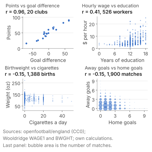
Each number measures the strength of a straight-line association: the clubs' points rise almost in step with goal difference, while wages, though higher on average with more education, are widely spread at every level. A correlation is not a slope: for the clubs it is 0.96, while the least-squares line of lesson 9 rises 0.62 points per goal of goal difference, a number whose size depends on the units. Nor is a correlation a cause: all four measure association.
The two correlations of -0.15 come from different pictures. The births stand in columns, since 1,176 of the mothers reported no cigarettes and smokers reported round numbers; match scores sit on a grid of whole numbers. A correlation reduces a scatter to one number and leaves its shape out, so look at the scatter as well.
Zero correlation is not independence
If \(X\) and \(Y\) are independent, every joint probability is the product of the two marginal ones, so the double sum for \(E[XY]\) splits into two single sums:
$$ \begin{aligned} E[XY] &= \sum_x \sum_y xy\, P(X = x)\, P(Y = y) \\ &= E[X]\, E[Y] , \end{aligned} $$and the covariance is zero: independence implies zero covariance, and so zero correlation. The reverse fails. Let \(X\) be -1, 0 or 1 with probability 1/3 each, and \(Y = X^2\) (Figure 2).
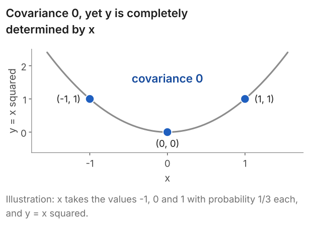
Then \(E[X] = 0\), \(E[Y] = 2/3\) and \(E[XY] = E[X^3]\), which is \((-1 + 0 + 1)/3 = 0\), so \(\operatorname{Cov}(X, Y) = 0 - 0 \times 2/3 = 0\). Yet \(Y\) is determined by \(X\): given \(X = 0\), \(Y\) is 0 for certain, although \(P(Y = 0) = 1/3\). The products of deviations, \((x - 0)(y - 2/3)\), are \(-1/3\), 0 and \(+1/3\) at \(x = -1\), 0 and 1: \(Y\) falls on the left and rises on the right, and the two halves cancel. A covariance, and so a correlation, measures straight-line association only; a relationship that bends can leave it at zero.
6. The variance of a sum
Total goals are home goals plus away goals, and a sample mean is a sum divided by \(n\), so we need the variance of a sum. For two random variables it is
$$ \begin{aligned} \operatorname{Var}(X + Y) = {} & \operatorname{Var}(X) + \operatorname{Var}(Y) \\ & + 2\operatorname{Cov}(X, Y) . \end{aligned} $$In words: variance of a sum = the sum of the variances plus twice the covariance.
Show the derivation of the variance of a sum
- Write the deviation of the sum. By section 3, \(X + Y\) has mean \(\mu_X + \mu_Y\), so its deviation is \(D_X + D_Y\), with \(D_X = X - \mu_X\) and \(D_Y = Y - \mu_Y\).
- Square it. $$ \begin{aligned} (D_X + D_Y)^2 = {} & D_X^2 + D_Y^2 \\ & + 2D_X D_Y . \end{aligned} $$
- Take expectations term by term, by the same rule: \(E[D_X^2] = \operatorname{Var}(X)\), \(E[D_Y^2] = \operatorname{Var}(Y)\) and \(E[2D_X D_Y] = 2\operatorname{Cov}(X, Y)\).
Intuitively, variables that move together reinforce each other's deviations, and their sum varies more; variables that move in opposite directions partly offset, and it varies less. The matches are the second case. Take them, as in sections 1 and 2, as the distribution, so that every variance and covariance divides by 1,900:
$$ 1.806 + 1.534 + 2 \times (-0.2546) = 2.831 , $$which is also the variance of the 1,900 totals worked out directly. Unrelated home and away goals would have given \(1.806 + 1.534 = 3.340\). The covariance is negative, so total goals vary less: a standard deviation of 1.68 goals rather than 1.83.
If \(X\) and \(Y\) are uncorrelated, and in particular if they are independent, the variances add. With more variables, the variance of a sum is the sum of the variances plus twice the covariance of every pair, and independence again makes every covariance zero. Lesson 6 uses two rules for the standard error, one from section 3 and one from the variance of a sum:
- A constant comes out of a variance squared: \(\operatorname{Var}(aX) = a^2\operatorname{Var}(X)\).
- The variance of a sum of independent random variables is the sum of their variances.
Under random sampling the observations \(X_1, \dots, X_n\) are independent draws from one distribution, each with variance \(\sigma^2\). So their sum has variance \(n\sigma^2\), and their mean \(\bar X\), the sum times \(1/n\), has variance \(n\sigma^2/n^2 = \sigma^2/n\); lesson 4 does this in full.
7. From the distribution to data: the sample versions
The mean \(\mu\), the variance \(\sigma^2\), the covariance and the correlation are fixed features of a distribution. From a sample of \(n\) observations, \(x_1, \dots, x_n\), we compute sample versions, which estimate them and vary from sample to sample:
$$ \bar x = \frac{1}{n}\sum_{i=1}^{n} x_i , $$ $$ s^2 = \frac{1}{n - 1}\sum_{i=1}^{n} (x_i - \bar x)^2 . $$In words: sample mean = sum of the observations divided by n; sample variance = sum of the squared deviations from the sample mean, divided by n - 1.
Its square root, \(s\), is the sample standard deviation. For pairs \((x_i, y_i)\), the sample covariance is the sum of the products of the deviations from \(\bar x\) and \(\bar y\), divided by \(n - 1\), and the sample correlation \(r\) divides it by the two sample standard deviations. The figures for the births, the workers and the clubs in sections 3 to 5 are of this kind.
Why divide by n - 1?
- What we are after. \(\sigma^2\), the average squared distance of an observation from the population mean \(\mu\).
- What we can measure. We do not know \(\mu\), so we measure distances from the sample mean \(\bar x\).
- Why those distances run small. \(\bar x\) is the number that makes the sum of squared distances from these \(n\) observations as small as it can be. So in every sample the squared distances from \(\bar x\) add to no more than those from \(\mu\).
- The shortfall. Under random sampling, their sum divided by \(n\) averages \((n - 1)\sigma^2/n\) across samples, not \(\sigma^2\).
- The correction. Dividing by \(n - 1\) removes the shortfall: \(s^2\) averages \(\sigma^2\) for any \(n\) of 2 or more, so it is unbiased.
Show where the factor (n - 1)/n comes from
- Split each distance from \(\mu\) in two. \(x_i - \mu = (x_i - \bar x) + (\bar x - \mu)\).
- Square and add over the \(n\) observations. The deviations from \(\bar x\) add to zero, so the cross term, \(2(\bar x - \mu)\sum_i (x_i - \bar x)\), vanishes, and $$ \begin{aligned} & \sum_{i=1}^{n} (x_i - \mu)^2 \\ &= \sum_{i=1}^{n} (x_i - \bar x)^2 + n(\bar x - \mu)^2 . \end{aligned} $$ The last term is never negative: this is step 3 above.
- Take expectations under random sampling, with the observations now random, \(X_1, \dots, X_n\). The left side averages \(n\sigma^2\), since each \((X_i - \mu)^2\) averages \(\sigma^2\). By section 3, \(X_1 + \dots + X_n\) has expectation \(n\mu\), so \(E[\bar X] = n\mu/n = \mu\): the sample mean is centred on \(\mu\). Hence the last term averages \(n\operatorname{Var}(\bar X) = n \times \sigma^2/n = \sigma^2\) (section 6).
- Subtract. The squared distances from \(\bar X\) add, on average, to \(n\sigma^2 - \sigma^2 = (n - 1)\sigma^2\). Divided by \(n\) they average \((n - 1)\sigma^2/n\); divided by \(n - 1\), \(\sigma^2\).
The count \(n - 1\) is called the degrees of freedom. The \(n\) deviations from \(\bar x\) add to zero, so once \(n - 1\) of them are known the last is fixed: one degree of freedom has gone into estimating the mean.
A simulation shows the shortfall. In 100,000 samples of 5 grades from a normal population with variance 100, dividing by \(n\) averaged 80.1 and dividing by \(n - 1\) averaged 100.1.
Show the simulation at 5, 25 and 100 grades
Grades are normal with mean 65 and variance 100. We draw \(R = 100{,}000\) samples of \(n\) grades and average both versions of the variance, and \(s\), over them; the table sets the averages beside the exact \(100(n - 1)/n\).
| Grades per sample, \(n\) | Divide by \(n\): average | Exact \(100(n - 1)/n\) | Divide by \(n - 1\): average | Average \(s\) |
|---|---|---|---|---|
| 5 | 80.1 | 80 | 100.1 | 9.41 |
| 25 | 95.9 | 96 | 99.9 | 9.89 |
| 100 | 99.1 | 99 | 100.1 | 9.98 |
Dividing by \(n\) falls a fifth short at \(n = 5\), 4% short at 25 and 1% short at 100, as the factor \((n - 1)/n\) says; dividing by \(n - 1\) averaged 100.1, 99.9 and 100.1 in this run.
In the same simulation \(s\) itself averaged 9.41 at \(n = 5\), a little below \(\sigma = 10\), although \(s^2\) averaged 100.1; at \(n = 100\) it averaged 9.98.
Show why \(s\) averages below \(\sigma\)
The square root pulls large values down more than small ones: 64 and 136 average 100, but their square roots, 8 and 11.66, average 9.83. So an average of square roots falls below the square root of the average, and \(s\) averages below \(\sigma\) although \(s^2\) averages \(\sigma^2\). For normal data an exact formula gives 9.40 at \(n = 5\), and the gap vanishes as \(n\) grows.
The code below prints the sample versions. Sections 1 to 6 took the 1,900 matches as the whole distribution; here they are a sample from the matches that sides like these could play. They are not a random sample, and treating them as independent draws is an approximation, since each club plays 38 matches a season. Their summary numbers are these:
| Home goals | Away goals | |
|---|---|---|
| Mean | 1.563 | 1.310 |
| Standard deviation | 1.344 | 1.239 |
| Covariance of the two | -0.2547 | |
| Correlation of the two | -0.153 | |
Stata: the code
import delimited "premier-league-matches-2019-24.csv", clear
summarize home_goals away_goals
correlate home_goals away_goals
correlate home_goals away_goals, covariance
Stata: what it prints
. summarize home_goals away_goals

    Variable |        Obs        Mean    Std. dev.       Min        Max
-------------+---------------------------------------------------------
  home_goals |      1,900    1.563158    1.344233          0          9
  away_goals |      1,900        1.31    1.238833          0          9

. correlate home_goals away_goals
(obs=1,900)

             | home_g~s away_g~s
-------------+------------------
  home_goals |   1.0000
  away_goals |  -0.1530   1.0000

. correlate home_goals away_goals, covariance
(obs=1,900)

             | home_g~s away_g~s
-------------+------------------
  home_goals |  1.80696
  away_goals | -.254713  1.53471
R: the code
# home and away goals per match: mean, sd, covariance, correlation
pl <- read.csv("premier-league-matches-2019-24.csv")
goals <- pl[, c("home_goals", "away_goals")]
sapply(goals, mean)
sapply(goals, sd)
cov(goals)
cor(goals)
R: what it prints
> # home and away goals per match: mean, sd, covariance, correlation
> pl <- read.csv("premier-league-matches-2019-24.csv")
> goals <- pl[, c("home_goals", "away_goals")]
> sapply(goals, mean)
home_goals away_goals
  1.563158   1.310000
> sapply(goals, sd)
home_goals away_goals
  1.344233   1.238833
> cov(goals)
           home_goals away_goals
home_goals   1.806962  -0.254713
away_goals  -0.254713   1.534708
> cor(goals)
           home_goals away_goals
home_goals   1.000000  -0.152955
away_goals  -0.152955   1.000000
Python: the code
import pandas as pd

# home and away goals per match: mean, sd, covariance, correlation
pl = pd.read_csv("premier-league-matches-2019-24.csv")
goals = pl[["home_goals", "away_goals"]]
print(goals.agg(["mean", "std"]))
print(goals.cov())
print(goals.corr())
Python: what it prints
      home_goals  away_goals
mean    1.563158    1.310000
std     1.344233    1.238833
            home_goals  away_goals
home_goals    1.806962   -0.254713
away_goals   -0.254713    1.534708
            home_goals  away_goals
home_goals    1.000000   -0.152955
away_goals   -0.152955    1.000000
The code reads premier-league-matches-2019-24.csv (1,900 matches: season, home, away, home_goals, away_goals, diff). Save it in your working folder first.
Stata, R and pandas divide by \(n - 1 = 1{,}899\), hence a covariance of -0.2547 here against -0.2546 in section 6, and a variance of home goals of 1.807 against 1.806. With 1,900 observations the divisor hardly matters; with five it does.
8. Common mistakes
- Reading a variance in the units of the data. The variance of home goals, 1.806, is in goals squared; the standard deviation, 1.344 goals, is in goals.
- Reading a covariance as a measure of strength. The same 526 workers give 4.151 with the wage in dollars and 415.1 with it in cents. Its sign says which way the two move together; its size depends on the units as well as on the association, so on its own it does not measure how closely.
- Reading a correlation as a slope. For the 20 clubs the correlation is 0.96 and the slope 0.62 points per goal: one measures how close the points lie to a line, the other how steep it is.
- "Zero correlation means independent." With \(X\) = -1, 0 or 1 and \(Y = X^2\), the covariance is zero, yet \(Y\) is determined by \(X\).
- "The variance of a sum is the sum of the variances." Only when the covariance is zero. For home and away goals, \(1.806 + 1.534 = 3.340\), but total goals have variance 2.831.
- Dividing by \(n\) and calling it the sample variance. Under random sampling, with five observations it averages 80% of \(\sigma^2\). Stata, R and pandas divide by \(n - 1\), numpy's
varby \(n\) unless givenddof=1; whichever you use, say which. - Confusing \(\mu\) with \(\bar x\). The population mean of home goals, 1.563, is fixed; samples of 10 matches gave means from 1.0 to 2.2.
9. Check your understanding
Five questions, marked on the page; every option has an explanation, including the wrong ones. (Without JavaScript the explanations are shown beneath each question.)
1. A household owns X cars, where P(X = 0) = 0.2, P(X = 1) = 0.5, P(X = 2) = 0.2 and P(X = 3) = 0.1. What is the expected number of cars, E[X]?
This divides 1.2 by 4, the number of values. The probabilities already do the averaging, since they add to 1: weight each value by its probability, add, and stop there.
1 is the most likely value, with probability 0.5. The expectation weights every value by its probability, and the chance of 2 or 3 cars pulls it above 1.
Correct. 0 × 0.2 + 1 × 0.5 + 2 × 0.2 + 3 × 0.1 = 0 + 0.5 + 0.4 + 0.3 = 1.2 cars. No household owns 1.2 cars: an expectation need not be a value the variable can take.
1.5 is the plain average of the values 0, 1, 2 and 3, as if each had probability 0.25. Here 0 and 1 together have probability 0.7, which pulls the expectation down to 1.2.
2. Five workers are paid £10, £12, £13, £16 and £19 an hour, with a standard deviation of £3.54. Each gets a rise of £1 an hour, and the new pay is recorded in pence. What is the standard deviation of the new figures?
This keeps the number it had in pounds. In pence every figure, every deviation from the mean and so the standard deviation are 100 times larger.
Correct. The new figure is 100 × (pay + 1) = 100 + 100 × pay. The added 100 pence moves every figure and the mean together, so it leaves the spread alone; the factor 100 multiplies every deviation, and so the standard deviation: 100 × 3.54 = 354 pence.
This adds the £1 rise, 100 pence, to the standard deviation. A rise for everyone moves every figure and the mean by the same amount, so the distances from the mean do not change.
This multiplies by 100 squared, the factor for the variance. The variance goes from 12.5 pounds squared to 125,000 pence squared; its square root, the standard deviation, rises only 100-fold, to 354.
3. For a sample of households, the covariance of weekly spending on food (in pounds) and household size (in people) is 18. The standard deviations are £40 and 1.5 people. What is the correlation?
Correct. 18/(40 × 1.5) = 18/60 = 0.3. The units of the covariance, pounds times people, cancel with those of the two standard deviations, and the result lies between -1 and 1, as every correlation does.
This is 18/40, dividing by the standard deviation of spending only. The result is still in people, not a pure number. Divide by both: 18/(40 × 1.5) = 0.3.
This is 18/1.5, dividing by the standard deviation of household size only. It is still in pounds, and a correlation cannot exceed 1. Divide by both: 18/60 = 0.3.
18 is the covariance itself, in pounds times people, and its size depends on those units. A correlation cannot exceed 1; dividing by both standard deviations gives 0.3.
4. X takes the values -2, -1, 1 and 2, each with probability 1/4, and Y = X squared. Then E[X] = 0 and E[XY] = E[X cubed] = 0, so the covariance of X and Y is 0. What follows?
Correct. Given X = 2, Y is 4 for certain, although P(Y = 4) = 1/2, so X and Y are not independent. With E[Y] = 2.5, the products of deviations, -3, 1.5, -1.5 and 3, cancel: a covariance picks up straight-line association only.
A zero covariance rules out a straight-line association, not every association. Independence would need P(Y = 4 given X = 2) to equal P(Y = 4) = 1/2; it is 1.
The average of Y given X is X squared: 4 when X is -2 or 2, and 1 when X is -1 or 1. It changes with X, although the covariance is zero.
5. A household's monthly spending on energy and on food, in pounds, have variances of 400 and 225 and a covariance of 30. What is the variance of its total spending on the two?
This subtracts twice the covariance, 625 - 60, which is the rule for a difference, energy minus food. For a sum the covariance is added: the two kinds of spending move together here.
This adds the two variances and leaves out the covariance, which is right only when the covariance is zero. Here it is 30, so the total varies more: 625 + 2 × 30 = 685.
This adds the covariance once. Squaring the sum of the two deviations gives their product twice, so the covariance enters twice: 400 + 225 + 2 × 30 = 685.
Correct. Var(X + Y) = Var(X) + Var(Y) + 2Cov(X, Y) = 400 + 225 + 60 = 685 pounds squared, a standard deviation of about £26.17.
10. Three questions about variance and correlation
The standard deviation is the square root of the variance. The variance is the average squared distance from the mean, in squared units: 1.806 goals squared for Premier League home goals. The square root returns it to goals, 1.344, a typical distance from the mean, though not the average distance, which is 1.082 goals.
Correlation is covariance divided by the two standard deviations. Both measure how two variables move together, but a covariance is in the product of their units and changes with them: for 526 workers' wages and education it is 4.15 in dollars and 415 in cents. The correlation is 0.41 either way, with no units, and always between -1 and 1.
Because the deviations are measured from the sample mean, which is closer to the data than the population mean, their squares add to less on average. Under random sampling, dividing by n gives (n - 1)/n of the population variance on average, a fifth short with 5 observations; dividing by n - 1 removes the shortfall.
11. Where next
- Lesson 4: sampling distributions, the law of large numbers and the central limit theorem: the sample mean as a random variable, its mean and variance found by the rules of this lesson.
- Lesson 5: standard deviation versus standard error: the spread of the data beside the spread of an estimate.
- Expectation, variance and covariance, the study notes: every rule in one table, with a portfolio example.
- Lesson 9: the OLS line by hand, where the slope of a regression line is a covariance divided by a variance.
- Lesson 2: random variables and distributions (previous) and the course home, which lists all 25 lessons and says which are published.
Stuck on a variance or covariance question? Send it
I tutor statistics and econometrics one-to-one, from a first expected value through to regression, panel data and time series. Bring the question you are stuck on and we will work through it in the free 30-minute consultation.
Book a free 30-minute consultation Econometrics tutor: how it works
Data and simulation. Matches: Premier League results from openfootball/england (CC0), seasons 2019/20 to 2023/24, 1,900 matches; the file the code reads is premier-league-matches-2019-24.csv. Clubs: the same source, final table of 2023/24. Wages: Wooldridge, Introductory Econometrics: A Modern Approach, data set WAGE1 (526 US workers, 1976). Births: the same book, data set BWGHT (1,388 births, 1988 National Health Interview Survey). Wooldridge results quoted, data not republished. Section 1, five samples of 10 matches: a fresh numpy default_rng(2026) and rng.choice(home_goals, size=(5, 10), replace=True), the home goals of the 1,900 matches in file order, one row per sample. Section 7, the divisor simulation: grades normal with mean 65 and standard deviation 10; for each n in 5, 25 and 100 a fresh numpy default_rng(2026) and rng.normal(65, 10, size=(100000, n)), filled row by row, one row per sample. The table of two 0/1 variables and the three-point example: illustrative. Adapted from my lecture notes for the MSc pre-sessional statistics course (ECON60901, 2015 and 2016) and for Time Series Econometrics (ECON30401) at the University of Manchester, and for Financial Econometrics (EC5609) at the University of St Andrews.