
A test's decision hides how close the call was: a sample mean of 68.3 rejects the claim that the mean grade is 65 or less, and 68.2 does not. The p-value is the probability, if the population mean were 65, of a sample mean at least as high as ours. Then we count how often a test decides wrongly.
In this lesson
- From a decision to a p-value
- What p-values look like when the null is true
- Two ways to be wrong: Type I and Type II errors
- Power: how often the test detects a false null
- The trade-off between the two errors
- More data: a smaller Type II error at the same level
- A small p-value is not a large difference
- Common mistakes
- Check your understanding: five marked questions
- Three questions about p-values and power
- Where next
1. From a decision to a p-value
Recall the test from lesson 7. Student A claims the mean grade is no more than 65; the null hypothesis is \(H_0: \mu \le 65\) and the alternative is \(H_1: \mu > 65\). Grades have standard deviation 10 and the sample has 25 students, so under random sampling the sample mean has a standard error of \(10/\sqrt{25} = 2\) (lesson 7; lesson 5 shows where \(\sigma/\sqrt{n}\) comes from). At the 5% level we reject H0 when the sample mean is above \(65 + 1.645 \times 2 = 68.29\).
A sample mean of 68.3 and one of 75 both give "reject", although the second is much stronger evidence. A sample mean of 68.2 gives "do not reject", although it is almost identical to 68.3. We would like a number that says how far into the tail the sample fell.
The p-value is that number. It answers the question: if the population mean were 65, the boundary of H0, in what share of samples would the sample mean be at least as far above 65 as the one we observed? Under random sampling from normal grades, the sample mean is then normal with mean 65 and standard error 2, so we standardise it (subtract 65 and divide by 2; lesson 2) and read the area from the standard normal distribution. As in lessons 6 and 7, a capital letter marks a quantity that varies from sample to sample (\(\bar X\) for the sample mean, \(Z\) for the standardised sample mean) and the lower-case letter the value our sample gives (lesson 2 sets out the notation). For a sample mean of 67:
$$ \begin{aligned} P(\bar X \ge 67 \mid \mu = 65) &= P\!\left(Z \ge \frac{67 - 65}{2}\right) \\ &= P(Z \ge 1) = 0.159 . \end{aligned} $$Read the bar as "when": the probability is calculated for a population in which \(\mu = 65\).
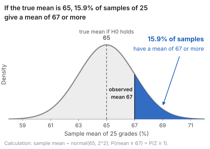
So a sample mean of 67 has a p-value of 0.159. If the population mean is 65, the boundary of Student A's claim, about one sample in six would give a mean of 67 or more; if it is below 65, fewer would. That is not rare, which is why the test did not reject.
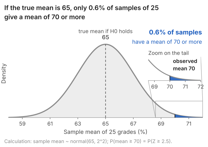
For a sample mean of 70 the same calculation gives \(P(Z \ge 2.5) = 0.006\). If the population mean is 65, only about one sample in 160 would give a mean of 70 or more, and if it is below 65, fewer would. That is rare, and the test rejected.
A p-value can also be found by counting. We drew 10,000 samples of 25 grades from a population in which the mean is 65, so that H0 is true by construction, and recorded the mean of each sample.
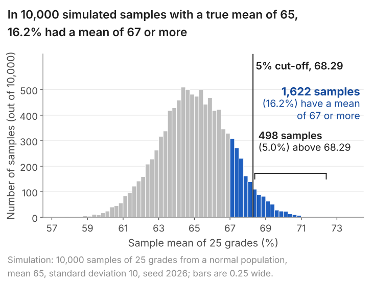
In the simulation 1,622 of the 10,000 sample means are 67 or more, a share of 16.2% against the 15.9% from the formula, and 63 are 70 or more, 0.6%.
Counting gives another way to read a p-value: it is a rank. Put the 10,000 simulated sample means in order from the largest down. A sample mean of 70 would stand about 63rd in the line, one of 68.29 about 498th and one of 67 about 1,622nd. The p-value is that position as a share of the line: 0.006, 0.05 and 0.16.
Definition: p-value
The p-value of a test is the probability, calculated on the assumption that the null hypothesis is true, of a test statistic at least as far from the null as the one observed.
Remarks. A small p-value means the data would be unusual if H0 were true, and so counts as evidence against H0. The p-value is NOT the probability that H0 is true. To find that probability we would also need to know how plausible H0 was before the data arrived, and the p-value does not use that.
The p-value and the decision rule of lesson 7 always agree. The cut-off 1.645 is the point with 5% of the area beyond it. If \(z\) is beyond the cut-off, the area beyond \(z\) is smaller than 5%. So "reject when \(z > 1.645\)" and "reject when the p-value is below 0.05" are the same rule. The p-value carries more information, because it lets the reader apply any level: 0.006 rejects at 5% and at 1%, and 0.159 rejects at neither.
For a two-tailed test, results far from H0 in either direction count, so the p-value is the area in both tails. For a sample mean of 67 that is \(2 \times 0.1587 = 0.317\).
What students say
“Nicky is an excellent econometrics tutor. He explains complex concepts clearly and makes them much easier to understand.”
“I was completely lost in my economics class, and then I started working Nicky and he totally saved me. He was excellent at explaining the material and extremely accommodating to meet with me many times despite us being in different time zones! Highly recommend working with Nicky!”
“Nicky is a very good and thorough teacher. He has excellent knowledge of econometrics and takes the time to work through your questions. Highly recommended!”
“Really great tutor! Encouraging, knowledgeable, friendly”
“Very good lesson, Nicky is very helpful.”
“Very helpful and clear.”
“I gather it was very useful, thank you!”
“Fantastic!”
2. What p-values look like when the null is true
Each of the 10,000 simulated samples has its own p-value. The top panel of Figure 4 shows all of them.
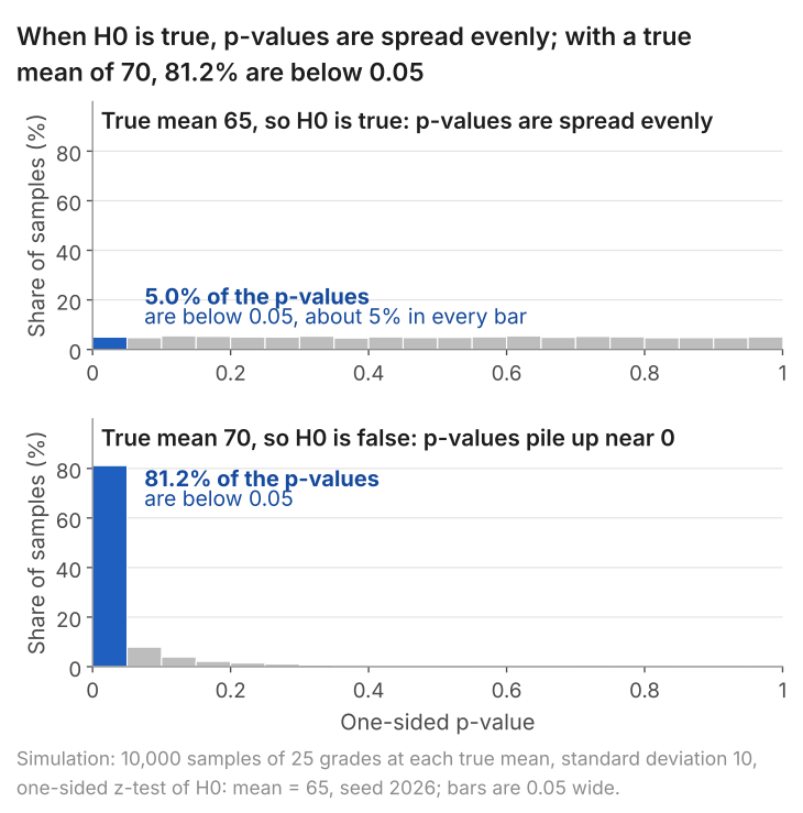
A p-value is a rank: the share of samples from a population with mean 65 whose sample mean is at least as large as ours. When the population mean really is 65, our sample is itself one draw from that population, so its rank is equally likely to fall anywhere from first to last. Hence the p-values are spread evenly between 0 and 1: a p-value below 0.05 is as likely as one between 0.50 and 0.55, and each range of width 0.05 holds about 5% of the samples. (If the mean were below 65, H0 would still be true, sample means would tend to be lower, and fewer than 5% of the p-values would fall below 0.05.)
In 498 of the 10,000 samples the p-value is below 0.05 and a 5% test rejects Student A's claim, although in this population his claim is true. The share of samples with that mistake, 5.0% here, is the simulation's estimate of the probability of rejecting a true H0, which at the boundary, 65, equals the significance level, 5%.
3. Two ways to be wrong: Type I and Type II errors
A test ends in one of two decisions, and the null hypothesis is either true or false. That gives four cases, two of which are mistakes.
| H0 is true | H0 is false | |
|---|---|---|
| Reject H0 | Type I error. Probability: at most the significance level, 5% here | Correct. Its probability is called the power (section 4) |
| Do not reject H0 | Correct. Probability: at least 95% here | Type II error. Probability: 1 minus the power |
The columns are the two possible states of the world, and we never know which one we are in. The rows are the two decisions. A Type I error is rejecting a null hypothesis that is true: the 498 samples of the last section. A Type II error is failing to reject a null hypothesis that is false.
The two error probabilities are fixed in different ways. The Type I probability is capped by us when we set the significance level: it is 5% when the mean is exactly 65, and smaller for any mean below 65. The Type II probability is not chosen. It depends on how far the true population mean is above 65, on the sample size and on the significance level, and it has to be worked out.
4. Power: how often the test detects a false null
Suppose Student A is wrong and the population mean is 70. Sample means are then normal with mean 70 and standard error 2, and the test still rejects when the sample mean is above 68.29. How often does that happen?
$$ \begin{aligned} & P(\bar X > 68.29 \mid \mu = 70) \\ &= P\!\left(Z > \tfrac{68.29 - 70}{2}\right) = P(Z > -0.855) \\ &= 0.804 . \end{aligned} $$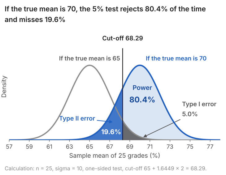
If the true mean is 70, the test rejects H0 in 80.4% of samples. That is its power against a mean of 70. In the other 19.6% of samples the sample mean happens to fall below 68.29, the test does not reject, and a Type II error is made. The bottom panel of Figure 4 is the same fact in the simulation: with a true mean of 70, 81.2% of the 10,000 p-values are below 0.05. (The simulated 81.2% differs from the exact 80.4% because 10,000 samples are themselves a sample. A share counted over \(R\) independent draws has standard error \(\sqrt{\text{share} \times (1 - \text{share})/R}\): the variance of one yes-or-no draw, divided by the number of draws, then square-rooted. Here that is \(\sqrt{0.8 \times 0.2/10{,}000} = 0.004\), or 0.4 percentage points, and the gap of 0.8 points is two standard errors.)
The power of this test depends on the true mean, so the table gives it for seven values:
| True mean | 65 | 66 | 67 | 68 | 69 | 70 | 72 |
|---|---|---|---|---|---|---|---|
| Probability of rejecting H0 | 5% | 13% | 26% | 44% | 64% | 80% | 97% |
| Probability of a Type II error | 87% | 74% | 56% | 36% | 20% | 3% |
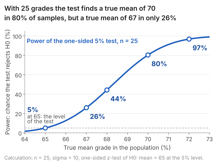
The table gives, for each possible true mean, the chance that the test rejects. At 65 that chance is the 5% significance level, since there H0 is true. If the true mean is 67, two marks above the claim, the test rejects in only 26% of samples: three times out of four it fails to detect that Student A is wrong. This is why "do not reject" could not be read as "Student A is right" in lesson 7. A sample of 25 is too small to tell a mean of 65 from a mean of 67 with any reliability.
5. The trade-off between the two errors
If a Type I error is a serious matter, we can make it rarer by testing at the 1% level. The standard normal distribution has 1% of its area above 2.326, so the cut-off for the sample mean moves up from \(65 + 1.645 \times 2 = 68.29\) to \(65 + 2.326 \times 2 = 69.65\). A true H0 is now rejected in at most 1% of samples, and in 1% when the mean is exactly 65.
The cost is paid in the other error. With the higher cut-off, fewer samples cross it when the true mean is 70 as well: power falls from 80% to 57%, and the Type II error probability rises from 20% to 43%.
| Significance level | Cut-off for the sample mean | Type I error | Power if the mean is 70 | Type II error if the mean is 70 |
|---|---|---|---|---|
| 5% | 68.29 | 5% | 80% | 20% |
| 1% | 69.65 | 1% | 57% | 43% |
With the sample size fixed, moving the cut-off reduces one error by increasing the other.
6. More data: a smaller Type II error at the same level
With the significance level held at 5%, more data leave the Type I error at 5% and cut the Type II error. More observations shrink the standard error, so the two curves of Figure 5 become narrower and overlap less, and a cut-off with 5% of the grey curve beyond it leaves less of the blue curve below it. (With enough data the level can be made stricter as well, and then both errors are smaller than before.)
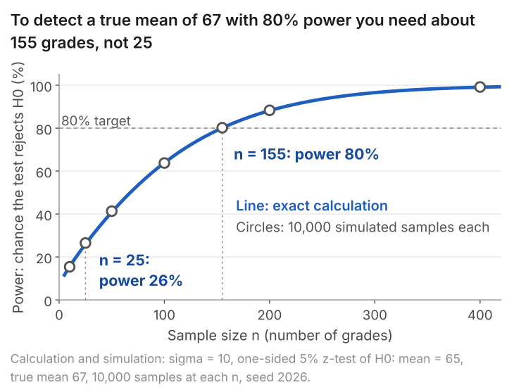
Against a true mean of 67, the test with 25 students has power of 26%. With 100 students it is 64%, and it takes 155 students to reach 80%. The significance level is 5% throughout.
In lesson 7 the test of no home advantage in the 2020/21 Premier League season did not reject. Could that test have detected an advantage of 0.3 goals a match? Three of the other four seasons showed 0.3 or more. The standard error was 0.097 goals. If the true advantage had been 0.3 goals a match, a test on 380 matches would have rejected in about 87% of samples. So the result is informative: an advantage of that size would probably have shown up. A "not significant" result from a test with power of 26% would tell us very little.
7. A small p-value is not a large difference
Power rises with the sample size against any alternative, including ones very close to H0. Suppose the true mean is 65.5 and we sample 10,000 students. The standard error is \(10/\sqrt{10{,}000} = 0.1\), a sample mean of 65.5 gives \(z = 5\), and the p-value is below 0.000001. The test rejects decisively, and it is right to: the mean is above 65. But it is above 65 by half a mark.
The p-value measures how unusual the sample would be if the population mean were 65. It does not measure how far the population mean is from 65. For the size of the difference, look at the estimate and its confidence interval.
A real case is in lesson 11. In the 1,388 births of lesson 6, a regression of birthweight on the number of cigarettes the mother smoked a day gives a slope with a p-value of about 2 in 100 million. The p-value says that a population slope of zero is ruled out at any conventional level. The size is read from the coefficient: 0.51 ounces lower per cigarette a day, which is 0.4% of the mean birthweight, or about 5 ounces at ten a day.
8. Common mistakes
- "The p-value is the probability that the null hypothesis is true." It is the probability of data at least this extreme, calculated on the assumption that the null is true.
- "I rejected at the 5% level, so there is a 5% chance I am wrong." The 5% is how often a true null is rejected. How likely a given rejection is to be a mistake also depends on the power and on how plausible the null was to begin with.
- "p is above 0.05, so the null is true." With a true mean of 67 and 25 students, the test fails to reject in 74% of samples.
- Mixing up the two errors. Type I: rejecting a true null. Type II: not rejecting a false one. The significance level sets the first directly. The second also depends on the true value and the sample size.
- Treating power as a single number. Power is always against a stated alternative: 26% against a mean of 67, 80% against 70.
- Reading a tiny p-value as a large effect. With 10,000 students a difference of half a mark gives a p-value below 0.000001.
9. Check your understanding
Five questions, marked on the page; every option has an explanation, including the wrong ones. (Without JavaScript the explanations are shown beneath each question.)
1. A one-sided test of H0: μ ≤ 65 gives a p-value of 0.159. What does 0.159 measure?
The probability that the null is true would also need how plausible the null was before the data were seen, and the p-value does not use that. It is the probability of a sample mean at least this large if the mean were 65.
Correct. It is the share of samples that would give a mean this far above 65, or further, if the true mean were 65: about one sample in six.
This is the same mistake in other words. The p-value describes how the data would behave under the null; it does not say how likely the null is.
2. If the null is true, the sample mean is normal with mean 65 and standard error 2. The sample mean is 69. Given P(Z > 1) = 0.159 and P(Z > 2) = 0.023, what is the one-sided p-value?
Correct. z = (69 - 65)/2 = 2, and the p-value is the area above 2: 0.023.
This doubles the tail area, which gives the two-sided p-value. The test here is one-sided.
0.159 is the area above z = 1. Here z = (69 - 65)/2 = 2.
0.977 is the area below z = 2. The p-value is the area in the direction of the alternative, above 2.
3. A test of H0: μ ≤ 65 is run at the 5% level. The true mean is in fact 70, and the sample leads to the decision "do not reject". What has happened?
A Type I error needs the null to be true and the decision to be 'reject'. Here the null is false and it was not rejected.
Correct. The null (a mean of 65 or less) is false, and the test failed to detect that. With n = 25 this happens in about 20% of samples when the true mean is 70.
Not rejecting is a decision, and it can be the wrong one. A test that misses a false null has made a Type II error.
4. With n = 25 the standard error of the sample mean is 2, and the test rejects when the sample mean exceeds 68.29. If the true mean is 66, what is the power of the test? Use P(Z > 1.145) = 0.126 and P(Z > 1.645) = 0.05.
0.05 is the area above the critical value 1.645, which is the probability of rejecting when the mean is 65. If the true mean is 66, sample means are centred on 66 and more of them fall above 68.29.
Correct. If the true mean is 66, the sample mean exceeds 68.29 when Z exceeds (68.29 - 66)/2 = 1.145, which has probability 0.126. The test misses a true mean of 66 in about seven samples out of eight.
The power would be 0.50 if the true mean were 68.29, the cut-off itself: half of the sample means would then fall above it. A true mean of 66 is 1.145 standard errors below the cut-off.
0.874 is the probability that the sample mean falls below 68.29, which is the Type II error. Power is the complement, 1 - 0.874.
5. The sample size stays at 25 and the significance level is cut from 5% to 1%. What happens to the probability of a Type I error when the mean is 65, and to the probability of a Type II error when the mean is 70?
Correct. The cut-off moves up from 68.29 to 69.65. Fewer samples cross it when the null is true, and fewer cross it when the true mean is 70 as well: power falls from 80% to 57%.
A stricter test rejects less often in every situation, including the ones where rejecting is right. With the sample size fixed, one error can be reduced only by raising the other.
The Type II error depends on the cut-off as well as on n. Moving the cut-off up to 69.65 means more samples from a population with mean 70 fall short of it.
10. Three questions about p-values and power
It means that, if the null hypothesis were true, a result at least as far from it as the one observed would occur in 5% of samples. It does not mean a 5% chance that the null is true, and it does not measure the size of the difference. Below 0.05, a result is called significant at the 5% level.
A Type I error is rejecting a null hypothesis that is true; its probability is at most the significance level, which the researcher chooses. A Type II error is failing to reject a null hypothesis that is false; its probability depends on the true value and the sample size. With the sample size fixed, lowering one raises the other.
Power is the probability that a test rejects the null hypothesis when a particular alternative is true. In the grade example, a one-tailed 5% test on 25 students has power of 80% against a true mean of 70 and 26% against 67. Power rises with the sample size and with the distance between the true mean and 65.
11. Where next
- Lesson 9: the OLS line by hand, the start of the regression part of the course. The tests and intervals of lessons 6 to 8 come back in lesson 11, applied to regression coefficients.
- Hypothesis testing explained, the explainer, which covers the same ground on one page.
- Confidence intervals and t-tests, for reporting the size of a difference and not only its p-value.
- Lesson 7: hypothesis tests step by step (previous) and the course home, which lists all 25 lessons and says which are published.
A p-value you cannot interpret? Send it
I tutor statistics and econometrics one-to-one, from a first hypothesis test through to regression, panel data and time series. Bring the result you are stuck on and we will work through it in the free 30-minute consultation.
Book a free 30-minute consultation Econometrics tutor: how it works
Simulations and data. Grades: a normal population with standard deviation 10; samples of 25 unless stated. Figures 3 and 4: 10,000 samples from a population with mean 65 (and, for the bottom panel of Figure 4, mean 70); for each simulation a fresh numpy default_rng(2026) and rng.normal(mean, 10, size=(10000, 25)), one row per sample; one-tailed z-test of H0: mean ≤ 65. Figure 7: exact power from the normal distribution, with 10,000 simulated samples at each of seven sample sizes. Birthweights: Wooldridge, Introductory Econometrics: A Modern Approach, data set BWGHT (1,388 births, 1988 National Health Interview Survey); results quoted, data not republished. Home advantage: openfootball/england (CC0), season 2020/21, 380 matches; the 87% is the power of a two-tailed 5% test against a true mean difference of 0.3 goals with a standard error of 0.097.