
Each coefficient in a regression printout estimates a population coefficient, and another sample would give another value. The standard error beside it estimates the typical distance between the two across samples; the t-statistic, p-value and confidence interval use it to say which population values the data rule out. We simulate this, build each number by hand, then read two printouts.
In this lesson
- A different sample gives a different line
- The standard error, built from the residuals
- From the standard error to t, p and the interval
- A real printout: 20 clubs
- A second printout: 1,388 births
- Common mistakes
- Check your understanding: five marked questions
- Three questions about the arithmetic
- Where next
1. A different sample gives a different line
In lessons 9 and 10 we fitted a line to five workers and found a slope of 2.2. Five other workers would have given a different slope. To say anything about the population the workers came from, we need to know how much the slope moves from one sample to the next. With real data we cannot find out directly, because we only have one sample. With a simulation we can.
Here is the recipe. The true line is y = 2 + 0.5x. Each sample has 30 points: x is drawn uniformly between 0 and 10, and y is the true line plus a random error drawn from a normal distribution with mean 0 and standard deviation 2. We draw 1,000 samples in this way and fit a least-squares line to each one.
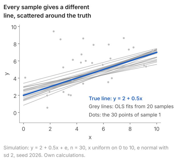
No grey line is the true line, and no two are the same. They are random, since each comes from a random sample, but they are centred on the true line: they fan out around it, above and below. Figure 2 collects the slopes of all 1,000 fitted lines.
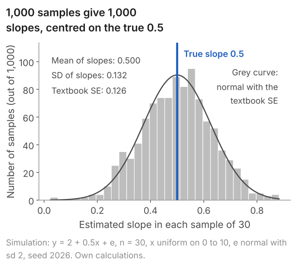
The slopes average 0.500, the true value: here, where the errors are unrelated to x, the method has no tendency to come out too high or too low. Their standard deviation is 0.132: the square root of the average squared distance between one sample's slope and the true slope, 0.5, so it reads as the typical distance between them. It is what we would like to know for a real regression.
In practice we cannot draw 1,000 samples. We have one. The standard error is an estimate of that standard deviation computed from the one sample we have. In the simulation the first sample on its own gives a slope of 0.405 and a standard error of 0.167. A researcher holding only that sample would report "0.4, give or take about 0.17", and the true 0.5 is well within that range.
Definition: standard error
The standard error of \(\hat\beta_1\) is an estimate, made from one sample, of the standard deviation that \(\hat\beta_1\) would have across repeated samples.
Remarks. The standard error is NOT the standard deviation of y or of x. Those describe how much the observations differ from each other. The standard error describes how much the estimate would differ from sample to sample, and it gets smaller as the sample gets larger.
What students say
“Nicky is an excellent econometrics tutor. He explains complex concepts clearly and makes them much easier to understand.”
“I was completely lost in my economics class, and then I started working Nicky and he totally saved me. He was excellent at explaining the material and extremely accommodating to meet with me many times despite us being in different time zones! Highly recommend working with Nicky!”
“Nicky is a very good and thorough teacher. He has excellent knowledge of econometrics and takes the time to work through your questions. Highly recommended!”
“Really great tutor! Encouraging, knowledgeable, friendly”
“Very good lesson, Nicky is very helpful.”
“Very helpful and clear.”
“I gather it was very useful, thank you!”
“Fantastic!”
2. The standard error, built from the residuals
How can one sample tell us how much the slope would vary across samples? The slope varies because of the errors: if every point lay exactly on the true line, every sample would give the same slope. So we need an estimate of how large the errors are, and the residuals provide it.
What we are after is how far the slope from one sample lies from the true slope across repeated samples. The measure is the variance of \(\hat\beta_1\) around \(\beta_1\): the average squared distance between them over repeated samples. Under random sampling, with nothing left in the errors that moves with x (so that \(\hat\beta_1\) is centred on \(\beta_1\), as in section 1), and with errors that have the same variance \(\sigma^2\) at every value of x, this variance is
$$ \operatorname{Var}(\hat\beta_1) = \frac{\sigma^2}{\sum (x_i - \bar x)^2} , $$treating the x values as given. The error variance is on top because the slope varies only because of the errors. The spread of x is underneath because a line held at points far apart is fixed more firmly than one held at points close together. A variance is in squared units, so we take the square root to return to the units of the slope, pounds an hour per year. We do not know \(\sigma\), so we put the residual standard error \(s\) in its place. For the five workers lesson 10 found
$$ s = \sqrt{\frac{\text{RSS}}{n-2}} = \sqrt{\frac{1.60}{3}} = 0.730 , $$and the sum of squared deviations of x from its mean is 4 + 1 + 0 + 1 + 4 = 10, so
$$ \begin{aligned} \text{se}(\hat\beta_1) &= \frac{s}{\sqrt{\sum (x_i - \bar x)^2}} \\ &= \frac{0.730}{\sqrt{10}} = 0.231 . \end{aligned} $$Before rounding the answer is 0.2309, and the t-statistic and the interval in section 3 use that figure so that they match the software.
In words: standard error of the slope = residual standard error divided by the square root of the sum of squared x deviations.
Each part of the formula makes sense by itself.
- More scatter around the line, larger standard error. If the points are far from the line (large \(s\)), many different lines fit almost as well, and the slope is uncertain.
- More spread in x, smaller standard error. If all the workers had nearly the same education, a small change in one pay figure could swing the slope a long way.
- More observations, smaller standard error. Each extra observation adds a term to \(\sum (x_i - \bar x)^2\), so the denominator grows with the sample.
Show where the variance of the slope comes from
- Write the slope in terms of the errors. Since \(\sum (x_i - \bar x)\bar y = 0\), the slope is \(\hat\beta_1 = \sum (x_i - \bar x) y_i / \sum (x_i - \bar x)^2\). Substitute \(y_i = \beta_0 + \beta_1 x_i + u_i\). The \(\beta_0\) term vanishes because \(\sum (x_i - \bar x) = 0\), and the \(\beta_1\) term gives \(\beta_1\) because \(\sum (x_i - \bar x) x_i = \sum (x_i - \bar x)^2\). So \(\hat\beta_1 = \beta_1 + \sum w_i u_i\), with weights \(w_i = (x_i - \bar x)/\sum (x_j - \bar x)^2\).
- Centre. If the errors have mean zero at every x, \(\hat\beta_1\) is centred on \(\beta_1\), so its variance is the average squared distance from \(\beta_1\).
- Independence lets the variances add. Under random sampling the errors are independent across observations, so \(\operatorname{Var}(\hat\beta_1) = \sum w_i^2 \operatorname{Var}(u_i)\).
- Same variance at every x. With \(\operatorname{Var}(u_i) = \sigma^2\) for every \(i\), \(\operatorname{Var}(\hat\beta_1) = \sigma^2 \sum w_i^2\) \(= \sigma^2 / \sum (x_i - \bar x)^2\).
3. From the standard error to t, p and the interval
The coefficient and its standard error are the main ingredients. The other three numbers in the row are calculated from them and from the degrees of freedom, n - 2. The t distribution used for the p-value and the interval is exact if the errors are normally distributed; five made-up points cannot tell us whether they are, so this example shows the mechanics.
- The t-statistic is the coefficient divided by its standard error: 2.2/0.2309 = 9.53. It says the estimate is about nine and a half standard errors away from zero. Zero is the comparison because a slope of zero would mean that pay does not differ with education at all.
- The p-value asks how often a t-statistic this far from zero would occur if the true slope were zero. For a t of 9.53 with 3 degrees of freedom the answer is 0.0025, about one sample in 400 (Stata and Python round it to 0.002). Data like ours would be very unusual if the true slope were zero. (Lesson 8 builds the p-value from first principles.)
- The 95% confidence interval is the coefficient plus and minus a multiple of the standard error. The multiple (the critical value of the t distribution) depends on the degrees of freedom, n - 2 = 3 here, and is read from a t table (the one below has it; lesson 6 explains where the multiple comes from): 3.182. So the interval is 2.2 ± 3.182 × 0.2309, which is 2.2 ± 0.7347, or 1.47 to 2.93. The 95% describes the method: intervals built in this way contain the true slope in 95% of samples (lesson 6 shows this for a mean). We can check this in the simulation of section 1: building a 95% interval from each of the 1,000 samples in the same way (the multiple is 2.048, with 28 degrees of freedom), 955 of the 1,000 intervals contain the true slope, 0.5.
In large samples the slope is approximately normal and the standard error is close to the standard deviation it estimates, so the multiple is the normal 1.96. With few observations the standard error is itself an uncertain estimate: with 3 degrees of freedom and normal errors, \(s\) comes out anywhere between about 0.34 and 1.61 times the true error standard deviation in 90% of samples. Intervals built when \(s\) is too small are too short and miss more often than they should; those built when \(s\) is too large miss less often, but the gain is smaller than the loss. So the multiple has to be larger to keep the 95% success rate. The table below gives it for several degrees of freedom.
| Degrees of freedom | 3 | 10 | 18 | 30 | 120 | Very large |
|---|---|---|---|---|---|---|
| Multiple for a 95% interval | 3.182 | 2.228 | 2.101 | 2.042 | 1.980 | 1.960 |
Software does all of this at once. Give it the five pairs and these are the results:
| Variable | Coefficient | Std. error | t | p-value | 95% interval |
|---|---|---|---|---|---|
| educ16 (the slope) | 2.2 | 0.2309 | 9.53 | 0.002 | 1.465 to 2.935 |
| constant | 9.6 | 0.5657 | 16.97 | 0.000 | 7.800 to 11.400 |
The whole regression: n = 5, R-squared = 0.968, root MSE = 0.730. Sums of squares: explained 48.4, residual 1.6, total 50.
Every number in the slope's row is one we have just computed: 2.2, 0.2309, 9.53, 0.002, and 1.47 to 2.93. The residual sum of squares is the 1.60 we started from, the total is the 50 from lesson 10, and R-squared is 1 - 1.60/50 = 0.968. The interval is wide: the line fits these five points very closely, and still the data are compatible with any slope from about £1.50 to £2.90 an hour per year.
The same results as each program prints them, with the commands that produce them:
Stata: the code
clear
input educ16 pay
0 10
1 12
2 13
3 16
4 19
end
regress pay educ16
Stata: what it prints
. regress pay educ16

      Source |       SS           df       MS      Number of obs   =         5
-------------+----------------------------------   F(1, 3)         =     90.75
       Model |        48.4         1        48.4   Prob > F        =    0.0025
    Residual |         1.6         3  .533333333   R-squared       =    0.9680
-------------+----------------------------------   Adj R-squared   =    0.9573
       Total |          50         4        12.5   Root MSE        =     .7303

------------------------------------------------------------------------------
         pay | Coefficient  Std. err.      t    P>|t|     [95% conf. interval]
-------------+----------------------------------------------------------------
      educ16 |        2.2   .2309401     9.53   0.002     1.465046    2.934954
       _cons |        9.6   .5656854    16.97   0.000     7.799737    11.40026
------------------------------------------------------------------------------
R: the code
# five made-up workers: years of education after 16 and hourly pay in pounds
workers <- data.frame(educ16 = c(0, 1, 2, 3, 4), pay = c(10, 12, 13, 16, 19))
fit <- lm(pay ~ educ16, data = workers)
summary(fit)
confint(fit)
anova(fit)
R: what it prints
> # five made-up workers: years of education after 16 and hourly pay in pounds
> workers <- data.frame(educ16 = c(0, 1, 2, 3, 4), pay = c(10, 12, 13, 16, 19))
> fit <- lm(pay ~ educ16, data = workers)
> summary(fit)

Call:
lm(formula = pay ~ educ16, data = workers)

Residuals:
   1    2    3    4    5
 0.4  0.2 -1.0 -0.2  0.6

Coefficients:
            Estimate Std. Error t value Pr(>|t|)
(Intercept)   9.6000     0.5657  16.971 0.000446 ***
educ16        2.2000     0.2309   9.526 0.002453 **
---
Signif. codes:  0 ‘***’ 0.001 ‘**’ 0.01 ‘*’ 0.05 ‘.’ 0.1 ‘ ’ 1

Residual standard error: 0.7303 on 3 degrees of freedom
Multiple R-squared:  0.968,	Adjusted R-squared:  0.9573
F-statistic: 90.75 on 1 and 3 DF,  p-value: 0.002453

> confint(fit)
               2.5 %    97.5 %
(Intercept) 7.799737 11.400263
educ16      1.465046  2.934954
> anova(fit)
Analysis of Variance Table

Response: pay
          Df Sum Sq Mean Sq F value   Pr(>F)
educ16     1   48.4  48.400   90.75 0.002453 **
Residuals  3    1.6   0.533
---
Signif. codes:  0 ‘***’ 0.001 ‘**’ 0.01 ‘*’ 0.05 ‘.’ 0.1 ‘ ’ 1
Python: the code
import pandas as pd
import statsmodels.formula.api as smf

# five made-up workers: years of education after 16 and hourly pay in pounds
workers = pd.DataFrame({"educ16": [0, 1, 2, 3, 4], "pay": [10, 12, 13, 16, 19]})
fit = smf.ols("pay ~ educ16", data=workers).fit()
print(fit.summary())
Python: what it prints
                            OLS Regression Results
==============================================================================
Dep. Variable:                    pay   R-squared:                       0.968
Model:                            OLS   Adj. R-squared:                  0.957
Method:                 Least Squares   F-statistic:                     90.75
Date:                Thu, 08 Oct 2026   Prob (F-statistic):            0.00245
Time:                        14:49:33   Log-Likelihood:                -4.2461
No. Observations:                   5   AIC:                             12.49
Df Residuals:                       3   BIC:                             11.71
Df Model:                           1
Covariance Type:            nonrobust
==============================================================================
                 coef    std err          t      P>|t|      [0.025      0.975]
------------------------------------------------------------------------------
Intercept      9.6000      0.566     16.971      0.000       7.800      11.400
educ16         2.2000      0.231      9.526      0.002       1.465       2.935
==============================================================================
Omnibus:                          nan   Durbin-Watson:                   1.725
Prob(Omnibus):                    nan   Jarque-Bera (JB):                0.641
Skew:                          -0.795   Prob(JB):                        0.726
Kurtosis:                       2.262   Cond. No.                         4.74
==============================================================================

Notes:
[1] Standard Errors assume that the covariance matrix of the errors is correctly specified.
The programs label the columns differently. Stata heads them Coefficient, Std. err., t, P>|t| and [95% conf. interval]. R heads them Estimate, Std. Error, t value and Pr(>|t|), and gives the interval separately with confint(fit). Python's statsmodels uses coef, std err, t, P>|t| and [0.025, 0.975]. The constant is _cons in Stata, (Intercept) in R and Intercept in Python.
4. A real printout: 20 clubs
Now the regression from lessons 9 and 10, points on goal difference (gd) for the 20 Premier League clubs of 2023/24.
| Variable | Coefficient | Std. error | t | p-value | 95% interval |
|---|---|---|---|---|---|
| gd | 0.6235 | 0.0408 | 15.29 | 0.000 | 0.538 to 0.709 |
| constant | 52.3 | 1.265 | 41.34 | 0.000 | 49.64 to 54.96 |
The whole regression: n = 20, R-squared = 0.9285, F(1, 18) = 233.77, root MSE = 5.658.
Stata: the code
import delimited "premier-league-2023-24.csv", clear
regress points gd
Stata: what it prints
. regress points gd

      Source |       SS           df       MS      Number of obs   =        20
-------------+----------------------------------   F(1, 18)        =    233.77
       Model |  7483.95222         1  7483.95222   Prob > F        =    0.0000
    Residual |  576.247782        18  32.0137657   R-squared       =    0.9285
-------------+----------------------------------   Adj R-squared   =    0.9245
       Total |      8060.2        19  424.221053   Root MSE        =    5.6581

------------------------------------------------------------------------------
      points | Coefficient  Std. err.      t    P>|t|     [95% conf. interval]
-------------+----------------------------------------------------------------
          gd |   .6234549   .0407763    15.29   0.000      .537787    .7091227
       _cons |       52.3   1.265183    41.34   0.000     49.64195    54.95805
------------------------------------------------------------------------------
R: the code
# Premier League 2023/24 final table: points (after deductions) and goal difference
pl <- read.csv("premier-league-2023-24.csv")
fit <- lm(points ~ gd, data = pl)
summary(fit)
confint(fit)
R: what it prints
> # Premier League 2023/24 final table: points (after deductions) and goal difference
> pl <- read.csv("premier-league-2023-24.csv")
> fit <- lm(points ~ gd, data = pl)
> summary(fit)

Call:
lm(formula = points ~ gd, data = pl)

Residuals:
   Min     1Q Median     3Q    Max
-9.078 -5.285  0.055  4.253  8.428

Coefficients:
            Estimate Std. Error t value Pr(>|t|)
(Intercept) 52.30000    1.26518   41.34  < 2e-16 ***
gd           0.62345    0.04078   15.29 9.36e-12 ***
---
Signif. codes:  0 ‘***’ 0.001 ‘**’ 0.01 ‘*’ 0.05 ‘.’ 0.1 ‘ ’ 1

Residual standard error: 5.658 on 18 degrees of freedom
Multiple R-squared:  0.9285,	Adjusted R-squared:  0.9245
F-statistic: 233.8 on 1 and 18 DF,  p-value: 9.356e-12

> confint(fit)
                2.5 %     97.5 %
(Intercept) 49.641949 54.9580511
gd           0.537787  0.7091227
Python: the code
import pandas as pd
import statsmodels.formula.api as smf

# Premier League 2023/24 final table: points (after deductions) and goal difference
pl = pd.read_csv("premier-league-2023-24.csv")
fit = smf.ols("points ~ gd", data=pl).fit()
print(fit.summary())
Python: what it prints
                            OLS Regression Results
==============================================================================
Dep. Variable:                 points   R-squared:                       0.929
Model:                            OLS   Adj. R-squared:                  0.925
Method:                 Least Squares   F-statistic:                     233.8
Date:                Thu, 08 Oct 2026   Prob (F-statistic):           9.36e-12
Time:                        14:49:35   Log-Likelihood:                -61.987
No. Observations:                  20   AIC:                             128.0
Df Residuals:                      18   BIC:                             130.0
Df Model:                           1
Covariance Type:            nonrobust
==============================================================================
                 coef    std err          t      P>|t|      [0.025      0.975]
------------------------------------------------------------------------------
Intercept     52.3000      1.265     41.338      0.000      49.642      54.958
gd             0.6235      0.041     15.290      0.000       0.538       0.709
==============================================================================
Omnibus:                        2.895   Durbin-Watson:                   1.352
Prob(Omnibus):                  0.235   Jarque-Bera (JB):                1.209
Skew:                          -0.004   Prob(JB):                        0.546
Kurtosis:                       1.795   Cond. No.                         31.0
==============================================================================

Notes:
[1] Standard Errors assume that the covariance matrix of the errors is correctly specified.
The code reads premier-league-2023-24.csv (20 rows: club, points, gd). Save it in your working folder first.
Read the row for gd from left to right.
- Coefficient, 0.623. Each extra goal of goal difference went with 0.62 more points. This is the slope we computed by hand in lesson 9.
- Standard error, 0.041. We can check it. Lesson 10 found a residual standard error of 5.658 (Root MSE in Stata, Residual standard error in R), and lesson 9 found the sum of squared goal differences to be 19,254. So the standard error is \(5.658/\sqrt{19{,}254} = 5.658/138.8 = 0.0408\).
- t, 15.29. The coefficient divided by its standard error, 0.62345/0.04078. The slope is more than fifteen standard errors from zero.
- p-value, 0.000. If the true slope were zero, a t-statistic this far from zero would occur in fewer than 5 samples in 10,000. The printed 0.000 is rounded, not exactly zero; R prints it as 9.36e-12, which means 9.36 × 10⁻¹².
- 95% interval, 0.538 to 0.709. With 18 degrees of freedom the multiple is 2.101: 0.6235 ± 2.101 × 0.0408.
The constant is the intercept, 52.3, the average points total. Its standard error can be checked too. Because the mean goal difference is zero, the intercept is the mean points total, and it differs from the true intercept only by the average of the 20 errors. So its standard error is the residual standard error divided by \(\sqrt{n}\), not the standard deviation of points divided by \(\sqrt{n}\): \(s/\sqrt{n} = 5.658/\sqrt{20} = 1.265\) points.
One caution about what the standard error means here. The 20 clubs are not a sample drawn from a larger population of clubs; they are the whole league for that season. The standard error answers a slightly different question in this case: how much the slope would be expected to differ if the same relationship between goal difference and points were observed in another season, with a different set of chance results. It also treats the 20 clubs' results as independent, which is an approximation, since every club plays every other club twice. The p-value and the interval are read in the same way. The next example is a sample in the ordinary sense.
5. A second printout: 1,388 births
The data are 1,388 US births recorded in the 1988 National Health Interview Survey. The dependent variable is birthweight in ounces, and cigs is the number of cigarettes the mother smoked a day during pregnancy.
| Variable | Coefficient | Std. error | t | p-value | 95% interval |
|---|---|---|---|---|---|
| cigs | -0.5138 | 0.0905 | -5.68 | 0.000 | -0.691 to -0.336 |
| constant | 119.77 | 0.572 | 209.27 | 0.000 | 118.65 to 120.89 |
The whole regression: n = 1,388, R-squared = 0.0227, F(1, 1386) = 32.24, root MSE = 20.13.
Stata: the code
* once: ssc install bcuse
bcuse bwght, clear
regress bwght cigs
Stata: what it prints
. regress bwght cigs

      Source |       SS           df       MS      Number of obs   =     1,388
-------------+----------------------------------   F(1, 1386)      =     32.24
       Model |  13060.4194         1  13060.4194   Prob > F        =    0.0000
    Residual |    561551.3     1,386  405.159668   R-squared       =    0.0227
-------------+----------------------------------   Adj R-squared   =    0.0220
       Total |   574611.72     1,387  414.283864   Root MSE        =    20.129

------------------------------------------------------------------------------
       bwght | Coefficient  Std. err.      t    P>|t|     [95% conf. interval]
-------------+----------------------------------------------------------------
        cigs |  -.5137721   .0904909    -5.68   0.000    -.6912861   -.3362581
       _cons |   119.7719   .5723407   209.27   0.000     118.6492    120.8946
------------------------------------------------------------------------------
R: the code
library(wooldridge)
data("bwght")
fit <- lm(bwght ~ cigs, data = bwght)
summary(fit)
confint(fit)
R: what it prints
> library(wooldridge)
> data("bwght")
> fit <- lm(bwght ~ cigs, data = bwght)
> summary(fit)

Call:
lm(formula = bwght ~ cigs, data = bwght)

Residuals:
    Min      1Q  Median      3Q     Max
-96.772 -11.772   0.297  13.228 151.228

Coefficients:
             Estimate Std. Error t value Pr(>|t|)
(Intercept) 119.77190    0.57234 209.267  < 2e-16 ***
cigs         -0.51377    0.09049  -5.678 1.66e-08 ***
---
Signif. codes:  0 ‘***’ 0.001 ‘**’ 0.01 ‘*’ 0.05 ‘.’ 0.1 ‘ ’ 1

Residual standard error: 20.13 on 1386 degrees of freedom
Multiple R-squared:  0.02273,	Adjusted R-squared:  0.02202
F-statistic: 32.24 on 1 and 1386 DF,  p-value: 1.662e-08

> confint(fit)
                  2.5 %      97.5 %
(Intercept) 118.6491529 120.8946479
cigs         -0.6912861  -0.3362581
Python: the code
import wooldridge
import statsmodels.formula.api as smf

bwght = wooldridge.data("bwght")
fit = smf.ols("bwght ~ cigs", data=bwght).fit()
print(fit.summary())
Python: what it prints
                            OLS Regression Results
==============================================================================
Dep. Variable:                  bwght   R-squared:                       0.023
Model:                            OLS   Adj. R-squared:                  0.022
Method:                 Least Squares   F-statistic:                     32.24
Date:                Thu, 08 Oct 2026   Prob (F-statistic):           1.66e-08
Time:                        14:49:36   Log-Likelihood:                -6135.5
No. Observations:                1388   AIC:                         1.227e+04
Df Residuals:                    1386   BIC:                         1.229e+04
Df Model:                           1
Covariance Type:            nonrobust
==============================================================================
                 coef    std err          t      P>|t|      [0.025      0.975]
------------------------------------------------------------------------------
Intercept    119.7719      0.572    209.267      0.000     118.649     120.895
cigs          -0.5138      0.090     -5.678      0.000      -0.691      -0.336
==============================================================================
Omnibus:                      118.187   Durbin-Watson:                   1.924
Prob(Omnibus):                  0.000   Jarque-Bera (JB):              635.742
Skew:                          -0.156   Prob(JB):                    8.92e-139
Kurtosis:                       6.301   Cond. No.                         6.72
==============================================================================

Notes:
[1] Standard Errors assume that the covariance matrix of the errors is correctly specified.
- Coefficient, -0.514. Each extra cigarette a day goes with a birthweight about half an ounce lower. The constant, 119.8 ounces, is the predicted weight for a non-smoker's baby.
- Standard error, 0.090, and t, -5.68. The slope is nearly six standard errors below zero. The sign of t is the sign of the coefficient. Significance depends on how far t is from zero, in either direction.
- p-value, 0.000. If the true slope were zero, a t-statistic as far from zero as -5.68 would occur in about 2 samples in 100 million.
- 95% interval, -0.691 to -0.336. With 1,386 degrees of freedom the multiple is 1.96. The interval lies entirely below zero, so the data rule out a slope of zero, and they are compatible with anything from about a third of an ounce to about 0.7 of an ounce per cigarette.
- R-squared, 0.0227. Cigarettes account for about 2% of the variation in birthweight. The Root MSE, 20.1 ounces, is almost as large as the standard deviation of birthweight itself, 20.4.
This regression has a slope that is clearly not zero together with a very low R-squared. The two statistics answer different questions. The t-statistic asks whether the slope can be told apart from zero, and 1,388 births are enough for that. R-squared asks how much of the variation in birthweight the line accounts for, and the answer is 2%: the other 98% differs between babies for reasons that are not in the regression. In one sentence: among these 1,388 births, each cigarette smoked a day during pregnancy is associated with a birthweight about half an ounce lower (95% confidence interval: 0.34 to 0.69 ounces lower), and smoking accounts for about 2% of the variation in birthweight.
The explainer on how to read regression output does the same for a regression with three explanatory variables, again with the Stata, R and Python code and output.
6. Common mistakes
- Treating the standard error as the standard deviation of the data. Birthweight has a standard deviation of 20.4 ounces. The slope's standard error is 0.090. They measure different things.
- Using 1.96 in a small sample. With five observations the multiple is 3.182, and 2.2 ± 1.96 × 0.231 would give an interval that is much too narrow.
- Dividing the wrong way round. t is the coefficient over the standard error, not the standard error over the coefficient.
- Reading P>|t| = 0.000 as zero. It is a rounded number. Write p < 0.001.
- Reading the p-value as the probability that the slope is zero. It is the probability of a t-statistic at least this extreme if the slope were zero.
- Taking a small p-value to mean a large effect. In the birthweight regression the p-value is tiny and R-squared is 0.023. Read the size from the coefficient and its units.
7. Check your understanding
Five questions, marked on the page; every option has an explanation, including the wrong ones. (Without JavaScript the explanations are shown beneath each question.)
1. A simple regression on 12 observations has a residual sum of squares of 40, and the sum of squared deviations of x from its mean is 25. What is the standard error of the slope?
2/25 = 0.08 divides by the sum of squared x deviations. The formula divides by its square root: 2/5 = 0.4.
This divides the residual sum of squares by n = 12: the square root of 40/12 is 1.83, and 1.83/5 = 0.37. Two parameters were estimated, so divide by n - 2 = 10.
Correct. The residual variance is 40/(12 - 2) = 4, so the residual standard error is 2. Dividing by the square root of 25 gives 2/5 = 0.40.
4/5 = 0.8 uses the residual variance, 4, where its square root, 2, is needed. The standard error is in the units of the slope, not their square.
2. A regression on 5 observations gives a slope of 2.2 with a standard error of 0.231. Software reports the 95% interval as 1.47 to 2.93, not 2.2 ± 1.96 × 0.231 = 1.75 to 2.65. Why?
Correct. 1.96 is the large-sample value. With n - 2 = 3 degrees of freedom the 95% critical value is 3.182, and 2.2 ± 3.182 × 0.2309 (the standard error before rounding) gives 1.47 to 2.93.
The interval printed is a 95% one. What changes with the sample size is the critical value for that level, because the standard error is itself estimated from few observations.
The standard error is the same 0.231 in both calculations. It is the multiple that changes: 3.18 with 3 degrees of freedom in place of 1.96.
3. For 1,388 births, the regression of birthweight (ounces) on cigarettes smoked a day gives a slope of -0.514 with a 95% confidence interval of -0.69 to -0.34. Which reading is correct?
The true slope is a fixed number; it is in this interval or it is not. The 95% describes the method: intervals built this way contain the true slope in 95% of samples.
The interval is about the uncertainty in one number, the average slope. It says nothing about how the relationship varies from mother to mother.
Correct. The 95% is the long-run success rate of the procedure. This particular interval, -0.69 to -0.34, is the range of slopes compatible with the data, and zero is well outside it.
4. In a sample of 1,388 births, birthweight has a standard deviation of 20.4 ounces and the regression slope on cigarettes has a standard error of 0.090. If the sample were four times larger, drawn in the same way, what would you expect?
The standard deviation describes how much babies differ from each other, and more data does not make babies more alike. Only the standard error shrinks.
Correct. The standard deviation is a feature of the population. The standard error measures the precision of the estimate and falls with the square root of the sample size: four times the data, half the standard error.
The standard error is not a description of the population. It describes how much the estimate varies across samples, and larger samples vary less.
5. In the birthweight regression the p-value for the slope on cigarettes is printed as 0.000 (in full, 0.00000002). Which statement is correct?
Correct. The p-value is computed assuming a true slope of zero, and gives the chance of a t-statistic at least as extreme as the one observed (-5.68). Here that chance is about 2 in 100 million.
The p-value is not the probability that the null hypothesis is true. It is the probability of data this extreme if the null were true, which is a different thing.
A small p-value says the slope is not zero, not that it explains much. R-squared in this regression is 0.023: cigarettes account for about 2% of the variation.
8. Three questions about the arithmetic
Add the squared residuals and divide by n - 2, then take the square root: that is the residual standard error. Divide it by the square root of the sum of squared deviations of x from its mean. For the five workers: the square root of 1.60/3 is 0.730, and 0.730 divided by the square root of 10 is 0.231.
Rounding. Software divides the unrounded coefficient by the unrounded standard error and then rounds the answer. If you divide two numbers that have already been rounded, the last digit can differ: 2.2/0.231 gives 9.52, while the software, using 0.2309, prints 9.53. Keep an extra decimal place in intermediate steps.
Use the t table with the regression's degrees of freedom: n - 2 for a simple regression, n - k - 1 with k explanatory variables. The value is 3.182 with 3 degrees of freedom, 2.101 with 18 and 1.980 with 120. It only reaches 1.96 in very large samples, where using 1.96 makes no practical difference.
9. Where next
- Lesson 12: multiple regression and "holding other things fixed": what each coefficient means when other regressors are in the model, shown on 526 US workers (1976).
- Confidence intervals and t-tests for what "95%" means, hypothesis testing explained for where a p-value comes from, and the t distribution for the multiples.
- R-squared and adjusted R-squared, for the fit statistics in the printout.
- Lesson 10: residuals, fit and R-squared (previous) and the course home, which lists all 25 lessons and says which are published.
Send me your output: module, question and deadline
I tutor econometrics one-to-one, from a first regression table through to panel data and time series. Bring the printout you are stuck on and we will read it together in the free 30-minute consultation.
Book a free 30-minute consultation Econometrics tutor: how it works
Data and simulation. Five-worker example: illustrative data. Simulation: y = 2 + 0.5x + e, 30 points a sample, x uniform on 0 to 10, e normal with mean 0 and standard deviation 2, 1,000 samples, numpy default_rng(2026), drawing the 30 x values and then the 30 errors for each sample in turn. Premier League: match results from openfootball/england (CC0), 2023/24 season, with the deductions for Everton (8 points) and Nottingham Forest (4 points) applied; the 20-row file the code reads is premier-league-2023-24.csv. Birthweight: Wooldridge, Introductory Econometrics: A Modern Approach, data set BWGHT (1,388 births, 1988 National Health Interview Survey), loaded with bcuse in Stata and with the wooldridge package in R and in Python; results quoted, data not republished.