Serial correlation (autocorrelation) means the error terms of a model are correlated across time instead of being white noise. In a time-series model it usually means the dynamics are misspecified and a higher-order model is needed. It is tested with the Breusch-Godfrey Lagrange multiplier test, which detects both AR and MA forms of residual correlation; the Durbin-Watson test should not be used once lagged dependent variables are present.
How to read these notes
These notes follow the serial-correlation section of a time-series econometrics course. They assume you have met OLS and the idea of AR and MA models, and that you know what white noise is. The aim is to explain why residual serial correlation is the central diagnostic in time-series modelling and how the standard test works in practice.
1. What serial correlation is
A regression model has the form \(y_t = x_t'\beta + u_t\), where the disturbance \(u_t\) collects everything not explained by the regressors. The standard assumption is that these disturbances are white noise: zero mean, constant variance, and — crucially — uncorrelated across time. When that last condition fails, so that \(\operatorname{Cov}(u_t, u_{t-k}) \neq 0\) for some lag \(k\), the disturbances are serially correlated (equivalently, autocorrelated).
The disturbances of a time-series model are serially correlated if they are correlated with their own past values, and hence are not white noise. Positive first-order serial correlation, where \(u_t\) tends to have the same sign as \(u_{t-1}\), is the most common case in economic data.
Intuitively, serial correlation means the model's mistakes are predictable: if it under-predicts this period, it tends to under-predict next period too. A correctly specified model should leave only unpredictable, white-noise residuals behind.
2. Why it matters: misspecified dynamics
In a time-series setting, the most important reason to care about serial correlation is what it reveals about the model. If the model does not account for all the dependence in the data, that leftover dependence shows up as serial correlation in the residuals — and the correct response is to use a richer model.
The point is sharp for autoregressive models. Suppose you fit an \(AR(p)\) but the true disturbances are themselves autocorrelated, following an \(AR(m)\) process rather than white noise:
where \(\varepsilon_t\) is white noise and \(L\) is the lag operator. Substituting the second equation into the first shows that the correct process for \(Y_t\) is actually an \(AR(p+m)\), not an \(AR(p)\). In other words, residual serial correlation is a signal that your specified model is too small — the dynamics are misspecified and a higher-order model is required.
This is why a serial-correlation test is treated as the headline diagnostic in time-series work: it directly answers the question "has my model captured all the dynamics, or is there predictable structure left over?"
There is also the inference cost familiar from cross-sectional work: even when the coefficients remain consistent, serially correlated errors make the usual standard errors wrong, so \(t\) and \(F\) tests are unreliable until the problem is addressed.
3. Good practice: always test after estimation
Because serial correlation carries this much information, it is good practice to apply a test for it after estimating any time-series model. A model that passes — leaving residuals with no significant serial correlation — is said to be dynamically complete: it has captured the systematic dynamics, and what remains is genuine random variation. A model that fails needs more lags.
4. The Breusch-Godfrey LM test
The standard tool is the Breusch-Godfrey test, a Lagrange multiplier (LM) test for residual autocorrelation. The recipe is an auxiliary regression. Having estimated the model and obtained residuals \(e_t\), regress those residuals on the original regressors plus \(m\) lags of the residuals:
The null hypothesis of no serial correlation is that the coefficients on all the lagged residuals are zero:
If the lagged residuals help predict the current residual, there is leftover serial correlation and we reject \(H_0\). The test statistic is asymptotically \(\chi^2_m\) under the null, although in practice an \(F\)-test of the same joint restriction is often preferred because it performs better in finite samples.
A valuable feature of the Breusch-Godfrey test is that it does not commit to a specific alternative: it has power against both \(AR(m)\) and \(MA(m)\) forms of residual correlation. It is a general test for the presence of serial correlation rather than a test of one particular model against another.
The usual guideline for choosing \(m\): use \(m=4\) for quarterly data and \(m=12\) for monthly data (to pick up any remaining seasonality), and \(m=1\) or \(2\) for annual data.
5. Why not the Durbin-Watson test?
Many software packages still report the Durbin-Watson statistic automatically, and many textbooks introduce it first. But it has a serious limitation: it only tests for first-order autocorrelation, and it does not account for the relationship between the regressors and lagged disturbances that arises whenever a lagged dependent variable is included — which is exactly the situation in any autoregressive or ARMA model.
In the context of an ARMA model the Durbin-Watson test is effectively useless and should not be used, nor its value reported, despite being printed by default. The Breusch-Godfrey LM test, by including the AR terms alongside the lagged residuals, does take proper account of this and is the correct choice.
6. A worked example: UK GDP growth
The logic comes alive on real data. For quarterly UK GDP growth, suppose an analyst first fits an \(MA(2)\) model. The estimated coefficients all look highly significant — but a Breusch-Godfrey test to lag \(m=4\) finds significant residual serial correlation at the 5% level. The \(MA(2)\) has not captured all the dynamics.
The shape of the correlogram (sample autocorrelations declining quickly from a positive first lag) instead suggests an \(AR(1)\). Re-estimating as an \(AR(1)\) gives a highly significant constant and AR coefficient, and this time the serial-correlation test finds no evidence of residual autocorrelation. The \(AR(1)\) is preferred: it is dynamically complete, whereas the \(MA(2)\) left predictable structure behind.
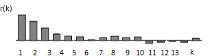 The correlogram of UK GDP growth suggests an AR(1); the serial-correlation test then confirms the AR(1) residuals are white noise while the MA(2) residuals are not.
The moral is that significance of the coefficients is not enough. A model is only adequate once its residuals pass the serial-correlation test — which is why, alongside information criteria such as AIC and BIC, the Breusch-Godfrey test is part of the standard model-checking routine.
Econometrics & time-series tuition
Serial-correlation testing trips up many students because the "obvious" test (Durbin-Watson) is the wrong one. For 1-1 help with the Breusch-Godfrey test, residual diagnostics or time-series model building, see econometrics tuition, statistics tuition or university economics tuition.
Free videos: the @economaths channel covers autocorrelation, testing for it and Newey-West standard errors.