
Before a match nobody knows the home side's goals, and before a birth nobody knows the baby's weight. To say in advance how likely an outcome is, we need the values such a number can take and their probabilities. A random variable is the uncertain number; its probability distribution gives the probability of each value or range of values.
In this lesson
- An outcome we cannot know in advance
- Random variables and notation
- Discrete random variables
- The cumulative distribution function
- Continuous random variables: probability is area
- The normal distribution and standardising
- Joint, marginal and conditional distributions
- Independence
- Common mistakes
- Check your understanding: five marked questions
- Three questions about random variables
- Where next
1. An outcome we cannot know in advance
The home side's goals in a Premier League match not yet played cannot be known in advance, but we can count the matches already played that ended with each number. The table counts the 1,900 matches of the five seasons 2019/20 to 2023/24 by home goals, and gives each count as a share of the 1,900, its relative frequency.
| Home goals | Matches | Relative frequency |
|---|---|---|
| 0 | 438 | 0.231 |
| 1 | 609 | 0.321 |
| 2 | 448 | 0.236 |
| 3 | 245 | 0.129 |
| 4 | 100 | 0.053 |
| 5 | 42 | 0.022 |
| 6 or more | 18 | 0.009 |
| All | 1,900 | 1 |
The shares are rounded to three decimals, so they add to 1.001; the working below uses the counts.
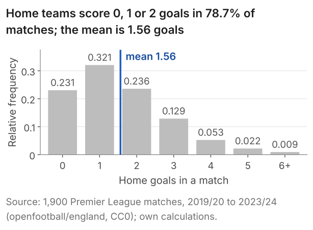
Initially it may seem odd to call such a number random: once a match is over, nothing about a home score of 2 is uncertain. Before kick-off, though, it was. Namely, there was some probability that the home side would score none, some probability of one, and so on, and if we could go back in time and replay the same fixtures we would see different scores. So we think of an observed score as one draw from a set of possible values, each with a probability attached.
To read a relative frequency as a probability, this lesson uses one device throughout: draw one of the 1,900 matches at random, each equally likely. The probability that the home side scored 2 goals in the match drawn is then \(448/1{,}900 = 0.236\). Whether 0.236 also holds for a match not yet played is a question about samples and populations, the subject of lesson 4.
What students say
“Nicky is an excellent econometrics tutor. He explains complex concepts clearly and makes them much easier to understand.”
“I was completely lost in my economics class, and then I started working Nicky and he totally saved me. He was excellent at explaining the material and extremely accommodating to meet with me many times despite us being in different time zones! Highly recommend working with Nicky!”
“Nicky is a very good and thorough teacher. He has excellent knowledge of econometrics and takes the time to work through your questions. Highly recommended!”
“Really great tutor! Encouraging, knowledgeable, friendly”
“Very good lesson, Nicky is very helpful.”
“Very helpful and clear.”
“I gather it was very useful, thank you!”
“Fantastic!”
2. Random variables and how we write them
To reason about the home side's goals before a match, we need a name for the uncertain number, separate from the value it will take.
Definition: random variable
A random variable is a number whose value is not known until it is observed. Formally, it is a rule that assigns a number to each possible outcome of something uncertain: to each way a match can end, the home side's goals.
Remarks. We write the random variable with a capital letter, \(X\) (the home side's goals before the match), and a value it can take with the lower-case letter, \(x\) (the 2 we saw afterwards). \(P(X = x)\) is read "the probability that \(X\) takes the value \(x\)"; for a match drawn from the 1,900, \(P(X = 2) = 0.236\). Books use other letters and write \(\Pr(X = x)\) or \(\Pr\{X = x\}\); the choice is cosmetic, since notation only shows which object is meant. \(X\) and \(x\) are not the same thing: \(X\) is uncertain and has a distribution, while \(x\) is one number.
A discrete random variable takes values that can be listed: goals (0, 1, 2, ...), or an outcome coded 0 or 1. A continuous one can take any value in a range: a birthweight, or an hourly wage.
The simplest discrete random variable has two values: \(X = 1\) if a person is employed and \(X = 0\) if not. With \(P(X = 1) = p\), and \(X\) certain to take one of its two values, \(P(X = 0) = 1 - p\). This is a Bernoulli random variable. A real one: in the 1988 National Health Interview Survey in the United States, 212 of the mothers of 1,388 babies smoked during pregnancy. Draw one birth at random and let \(S = 1\) if the mother smoked: \(P(S = 1) = 212/1{,}388 = 0.153\). On this page the 1,388 births are the whole population we draw from, so each probability about them is a share of the 1,388.
3. The distribution of a discrete random variable
For a discrete random variable, a complete description of the uncertainty about \(X\) is a list of every value \(X\) can take with its probability, the probability distribution of \(X\). The rule that gives the probability of each value is the probability function:
$$ f(x) = P(X = x) . $$In words: the probability function at \(x\) is the probability that \(X\) takes the value \(x\).
It is also called the probability mass function, and some books say density even when \(X\) is discrete, a word this lesson keeps for section 5. For home goals, the relative frequencies of section 1 give \(f(0) = 0.231\), \(f(1) = 0.321\), and so on.
Each \(f(x)\) here is a share of the 1,900 matches (a count between 0 and 1,900, divided by 1,900), so it lies between 0 and 1, as every probability does. And \(X\) must take one of its values: the counts add to 1,900, so the probabilities add to 1.
$$ 0 \le f(x) \le 1 \quad\text{and}\quad \sum_x f(x) = 1 . $$In words: each probability is between 0 and 1, and the probabilities of all the values add to 1.
A match cannot end with both 0 and 1 home goals, so the probability that \(X\) takes one value or the other is the sum of their probabilities. The probability of at most 1 home goal is
$$ \begin{aligned} P(X \le 1) &= f(0) + f(1) \\ &= \frac{438 + 609}{1{,}900} = 0.551 , \end{aligned} $$and of 3 or more, from the 245 + 100 + 42 + 18 = 405 matches with 3 or more home goals, \(405/1{,}900 = 0.213\).
4. The cumulative distribution function
Questions such as the probability of at most 2 home goals, or of 1 to 3, are answered by the cumulative distribution function, which gives, at any number \(x\), the probability that \(X\) is no larger than \(x\):
$$ F(x) = P(X \le x) . $$In words: the cumulative distribution function at \(x\) is the probability that \(X\) is \(x\) or less.
For a discrete random variable it is a running total of the probability function. The table keeps the running total in matches, so that nothing is lost to rounding, and divides it by 1,900.
| Home goals \(x\) | Matches | Matches with \(x\) or fewer | \(F(x)\) |
|---|---|---|---|
| 0 | 438 | 438 | 0.231 |
| 1 | 609 | 1,047 | 0.551 |
| 2 | 448 | 1,495 | 0.787 |
| 3 | 245 | 1,740 | 0.916 |
| 4 | 100 | 1,840 | 0.968 |
| 5 | 42 | 1,882 | 0.991 |
| 6 | 11 | 1,893 | 0.996 |
| 7 | 4 | 1,897 | 0.998 |
| 8 | 1 | 1,898 | 0.999 |
| 9 | 2 | 1,900 | 1 |
Stata: the code
import delimited "premier-league-matches-2019-24.csv", clear
tabulate home_goals
Stata: what it prints
. tabulate home_goals

 home_goals |      Freq.     Percent        Cum.
------------+-----------------------------------
          0 |        438       23.05       23.05
          1 |        609       32.05       55.11
          2 |        448       23.58       78.68
          3 |        245       12.89       91.58
          4 |        100        5.26       96.84
          5 |         42        2.21       99.05
          6 |         11        0.58       99.63
          7 |          4        0.21       99.84
          8 |          1        0.05       99.89
          9 |          2        0.11      100.00
------------+-----------------------------------
      Total |      1,900      100.00
R: the code
# home goals per match, 1,900 Premier League matches (2019/20 to 2023/24)
pl <- read.csv("premier-league-matches-2019-24.csv")
counts <- table(pl$home_goals)
share <- prop.table(counts)
round(cbind(count = counts, share, cumulative = cumsum(share)), 4)
R: what it prints
> # home goals per match, 1,900 Premier League matches (2019/20 to 2023/24)
> pl <- read.csv("premier-league-matches-2019-24.csv")
> counts <- table(pl$home_goals)
> share <- prop.table(counts)
> round(cbind(count = counts, share, cumulative = cumsum(share)), 4)
  count  share cumulative
0   438 0.2305     0.2305
1   609 0.3205     0.5511
2   448 0.2358     0.7868
3   245 0.1289     0.9158
4   100 0.0526     0.9684
5    42 0.0221     0.9905
6    11 0.0058     0.9963
7     4 0.0021     0.9984
8     1 0.0005     0.9989
9     2 0.0011     1.0000
Python: the code
import pandas as pd

# home goals per match, 1,900 Premier League matches (2019/20 to 2023/24)
pl = pd.read_csv("premier-league-matches-2019-24.csv")
goals = pl["home_goals"]
counts = goals.value_counts(sort=False).sort_index()
share = goals.value_counts(sort=False, normalize=True).sort_index()
table = pd.DataFrame({"count": counts, "share": share,
                      "cumulative": share.cumsum()})
print(table.round(4))
Python: what it prints
            count   share  cumulative
home_goals
0             438  0.2305      0.2305
1             609  0.3205      0.5511
2             448  0.2358      0.7868
3             245  0.1289      0.9158
4             100  0.0526      0.9684
5              42  0.0221      0.9905
6              11  0.0058      0.9963
7               4  0.0021      0.9984
8               1  0.0005      0.9989
9               2  0.0011      1.0000
The code reads premier-league-matches-2019-24.csv (1,900 matches: season, home, away, home_goals, away_goals, diff). Save it in your working folder first.
The row for 2 goals gives \(F(2) = 1{,}495/1{,}900 = 0.787\): in 78.7% of the matches the home side scored 2 goals or fewer. For "between", the matches with 3 or fewer goals are those with none plus those with 1 to 3, so \(F(3) = F(0) + P(1 \le X \le 3)\), and
$$ \begin{aligned} P(1 \le X \le 3) &= F(3) - F(0) \\ &= 0.916 - 0.231 = 0.685 . \end{aligned} $$In words: the probability of 1 to 3 goals is the probability of 3 or fewer minus the probability of none.
One goal is inside the range, so we subtract \(F(0)\), not \(F(1)\). The running total reaches all 1,900 matches at 9 goals, the highest home score in the data, so \(F(9) = 1\): every match had 9 or fewer. Above 9, \(F\) stays at 1.
5. Continuous random variables: probability is area
What replaces the probability function when a random variable can take any value in a range? Take birthweight. A weight of exactly 120 ounces means 120.000... to every decimal place, so a baby of 120.01 ounces does not count. The narrower the range we allow around 120, the smaller the share of babies in it, and for a continuous random variable the share shrinks to zero as the width does. A single value is a range of width zero, so each single value has probability zero; probabilities belong to ranges.
The survey records weights in whole ounces, so the 13 babies recorded at 100 ounces stand for a range of true weights near 100, not for one value.
In place of a probability function, a continuous random variable has a density \(f(x)\): a curve drawn so that the area under it over any range is the probability of that range. \(X\) must take some value, so the whole area is 1. For any two numbers \(a\) and \(b\),
$$ P(a \le X \le b) = \int_a^b f(x)\,dx . $$In words: the probability that \(X\) lies between \(a\) and \(b\) is the area under the density between them (the integral is the name for that area).
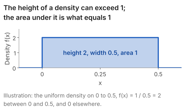
So a density is not a probability. An area is a height times a width, so a density is probability per unit of \(x\), per ounce for a birthweight. If the values lie within a range less than one unit wide, the density must be higher than 1 somewhere for the area to reach 1. In Figure 2 the height is 2, and the probability of a value between 0.1 and 0.2 is the area \(2 \times 0.1 = 0.2\).
With data, a histogram drawn on the density scale plays the part of the density. In Figure 3 the 1,388 birthweights are in bars 10 ounces wide, and each bar's height is its share of births divided by 10 ounces, so that its area is that share. The tallest bar, from 120 up to 130 ounces, holds 297 births, a share of 0.214, so its height is 0.0214 per ounce. The blue curve is a normal density, for section 6.
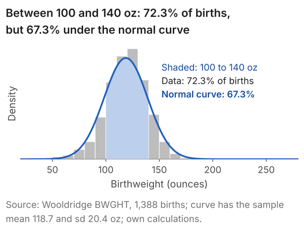
For a birth drawn at random from the 1,388, the probability that it weighs at least 100 ounces and under 140 is the area of the four bars from 100 to 140: \(994/1{,}388 = 0.716\).
6. The normal distribution and standardising
One continuous distribution, the normal, has a section to itself because of a result about sample means. Under random sampling (each observation drawn independently from the same population), and provided the variance of the data is finite, the distribution of the sample mean is approximately normal in large samples, whatever the shape of the distribution of the data. This is the central limit theorem of lesson 4. Hence the large-sample probabilities of lessons 6 to 8 are areas under a normal curve, and the multiples 1.96 and 1.645 are points of the standard normal distribution, found below.
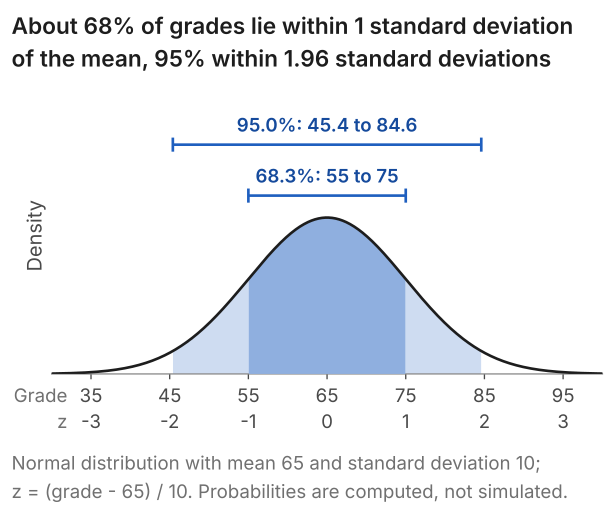
A normal distribution has a bell-shaped density, symmetric about its centre and fixed by two numbers: the mean \(\mu\), its centre, and the standard deviation \(\sigma\), its spread. We write \(X \sim N(\mu, \sigma^2)\); the second number is the variance, the square of \(\sigma\). The example of lessons 6 to 8 is exam grades, normal with mean 65 and standard deviation 10: \(N(65, 100)\).
What we are after is the probability of any range, for any mean and standard deviation, from one table or one function in software. The step is to standardise:
$$ Z = \frac{X - \mu}{\sigma} . $$In words: Z = (value minus the mean) divided by the standard deviation.
Subtracting \(\mu\) moves the centre to 0: a grade of 75 becomes 10 marks above the mean. Dividing by \(\sigma\) measures that distance in standard deviations, so \(z = (75 - 65)/10 = 1\). The marks cancel, so \(Z\) has no units. If \(X\) is normal, \(Z\) is normal with mean 0 and standard deviation 1, whatever \(\mu\) and \(\sigma\) are: the standard normal distribution, \(N(0, 1)\), with \(Z\) the random variable and \(z\) a value it takes. Hence one table of the standard normal serves every normal distribution.
Show why the standardised variable has mean 0 and standard deviation 1
- Mean. \(Z = X/\sigma - \mu/\sigma\). Multiplying a random variable by a constant multiplies its mean by it, and subtracting a constant subtracts it from the mean, so the mean of \(Z\) is \(\mu/\sigma - \mu/\sigma = 0\).
- Standard deviation. Subtracting a constant leaves the spread unchanged, and multiplying by \(1/\sigma\) divides the standard deviation by \(\sigma\), giving \(\sigma/\sigma = 1\).
- Shape. A shifted and rescaled normal random variable is normal. Only this step needs \(X\) to be normal: standardising any random variable whose standard deviation exists and is not zero gives mean 0 and standard deviation 1.
The rules used in steps 1 and 2 are in lesson 3.
Software, or a printed table, gives \(P(Z \le 1) = 0.8413\) for the standard normal. So for the grades
$$ \begin{aligned} P(X > 75) &= P(Z > 1) \\ &= 1 - 0.8413 = 0.159 . \end{aligned} $$In words: 15.9% of grades are more than one standard deviation above the mean.
The density is symmetric, so another 15.9% lie below 55, which leaves \(1 - 2 \times 0.1587 = 0.683\) between 55 and 75. In the same way, the standard normal has 2.5% of its area above 1.96 and 2.5% below -1.96, so 95% of grades lie within 1.96 standard deviations of the mean, between
$$ \begin{aligned} 65 - 1.96 \times 10 &= 45.4 \;\text{ and} \\ 65 + 1.96 \times 10 &= 84.6 . \end{aligned} $$That is where the 1.96 of lesson 6 comes from. Likewise 1.645 is the point with 5% of the area beyond it, the cut-off of the one-tailed test in lesson 7.
Real data are only approximately normal. Of the 1,388 births, 72.3% lie within one standard deviation of the mean, from 98.35 to 139.05 ounces, where a normal curve with the same mean and standard deviation has 68.3%. Figure 3's range, 100 to 140 ounces, is slightly different: it holds 72.3% of the births too, but 67.3% of the area under the curve. Nine births lie more than three standard deviations below the mean, where the curve has 1.9. Within 1.96 standard deviations the two agree, 95.2% against 95.0%. So the normal curve is an approximation to these data, close at the 95% mark and poor in the lower tail, and whether it is good enough depends on the use.
Show the births against the normal curve, range by range
The table sets the share of the 1,388 births in four ranges beside the area over the same range under the normal curve with the births' mean (118.7 ounces) and standard deviation (20.35 ounces).
| Range | Weights (ounces) | Births | Share of births | Normal curve |
|---|---|---|---|---|
| Within 1 standard deviation of the mean | 98.35 to 139.05 | 1,003 | 72.3% | 68.3% |
| Within 1.96 standard deviations | 78.81 to 158.59 | 1,321 | 95.2% | 95.0% |
| More than 3 standard deviations below | under 57.65 | 9 | 0.65% | 0.13% |
| More than 3 standard deviations above | over 179.75 | 2 | 0.14% | 0.13% |
One of the 9 births in the lower tail is recorded at 23 ounces. In the upper tail the data and the curve agree, 2 births against 1.9.
7. Two random variables at once: joint, marginal and conditional distributions
Economics is about relationships, such as whether a mother's smoking goes with a lighter baby, and a relationship needs the distribution of both variables at once. Start with made-up probabilities for \(X\) and \(Y\), each 0 or 1: each inner cell is the probability of one pair of values, and the margins hold the row and column totals.
| \(Y = 0\) | \(Y = 1\) | \(P(X = x)\) | |
|---|---|---|---|
| \(X = 0\) | 0.4 | 0.3 | 0.7 |
| \(X = 1\) | 0.1 | 0.2 | 0.3 |
| \(P(Y = y)\) | 0.5 | 0.5 | 1 |
The four inner cells are the joint probability function:
$$ f(x, y) = P(X = x, Y = y) . $$In words: the probability that \(X\) takes the value \(x\) and \(Y\) the value \(y\).
So \(P(X = 1, Y = 1) = 0.2\), and the four cells add to 1. \(X = 0\) happens either with \(Y = 0\) or with \(Y = 1\), never both, so adding along its row gives \(P(X = 0) = 0.4 + 0.3 = 0.7\). In general,
$$ f_X(x) = P(X = x) = \sum_y f(x, y) . $$In words: the probability that \(X = x\) is the sum of the joint probabilities in its row.
This is the marginal distribution of \(X\), named for where it sits, in the margin of the table; the subscript in \(f_X\) says which variable it belongs to. The column totals give the marginal distribution of \(Y\).
Now suppose we learn that \(X = 1\). Only the bottom row remains possible, and its probabilities, 0.1 and 0.2, add to 0.3. Dividing each by 0.3 makes them add to 1 and gives the distribution of \(Y\) among the cases where \(X = 1\): the conditional distribution of \(Y\) given \(X = 1\). Provided \(P(X = x)\) is not zero,
$$ P(Y = y \mid X = x) = \frac{f(x, y)}{f_X(x)} . $$In words: conditional probability = joint probability divided by the probability of the condition.
The bar is read "given". Here \(P(Y = 1 \mid X = 1) = 0.2/0.3 = 0.667\), but \(P(Y = 1 \mid X = 0) = 0.3/0.7 = 0.429\).
The births give a real table. Draw one of the 1,388 at random; let \(S = 1\) if the mother smoked and \(L = 1\) if the baby weighed under 2,500 grams (88.18 ounces), the standard definition of low birthweight. Each cell gives the count and, in brackets, the joint probability: the count divided by 1,388.
| \(L = 1\) (low) | \(L = 0\) | All | |
|---|---|---|---|
| \(S = 1\) (smoked) | 21 (0.015) | 191 (0.138) | 212 (0.153) |
| \(S = 0\) | 67 (0.048) | 1,109 (0.799) | 1,176 (0.847) |
| All | 88 (0.063) | 1,300 (0.937) | 1,388 (1) |
In the conditional probability the 1,388s cancel, leaving a share of the 212 smokers:
$$ \begin{aligned} P(L = 1 \mid S = 1) &= \frac{21/1{,}388}{212/1{,}388} \\ &= \frac{21}{212} = 0.099 , \end{aligned} $$against \(67/1{,}176 = 0.057\) for the babies of mothers who did not smoke. That is an association in these births, not a finding that smoking causes low birthweight: mothers who smoked may have differed in other ways too.
8. Independence
Two random variables can be unrelated in a precise sense: learning the value of one tells us nothing about the other. \(X\) and \(Y\) are independent if knowing the value of \(X\) does not change the distribution of \(Y\). For every \(x\) and \(y\),
$$ P(Y = y \mid X = x) = P(Y = y) . $$In words: whatever value \(X\) takes, the conditional distribution of \(Y\) is its marginal distribution.
Multiplying both sides by \(P(X = x)\) turns the left side into the joint probability, which gives the form that is easier to check in a table. For every \(x\) and \(y\),
$$ f(x, y) = f_X(x)\, f_Y(y) . $$In words: under independence every inner cell equals its row total times its column total.
One failing cell is enough to rule independence out, for probabilities as here; in a sample, shares miss the products by chance even under independence, so a test is needed. In the made-up table \(P(X = 0) \times P(Y = 0)\) is \(0.7 \times 0.5 = 0.35\), not the 0.4 in that cell, so \(X\) and \(Y\) are not independent. Nor are \(S\) and \(L\): \(P(S = 1) \times P(L = 1)\) is \(0.1527 \times 0.0634 = 0.0097\) (to four decimals), against a joint probability of 0.0151.
Independence is part of random sampling, the assumption on which lessons 4 to 8 build: the \(n\) observations of a sample, written \(X_1, \dots, X_n\) before it is drawn, are independent draws from one distribution, so the first birthweight in a sample tells us nothing about the second. Lesson 4 uses that independence to show that the variance of the sample mean is \(\sigma^2/n\).
Independent is not the same as mutually exclusive. Let \(H = 1\) if the home side wins and \(D = 1\) if the match is drawn. No match is both, so \(P(H = 1, D = 1) = 0\), while the product of the two marginal probabilities is \(0.441 \times 0.227 = 0.100\). So \(H\) and \(D\) are dependent: learning that the home side won tells us the match was not drawn. Outcomes that cannot happen together are dependent whenever each has a positive probability.
9. Common mistakes
- Reading a density as a probability. The uniform density on 0 to 0.5 has height 2; probabilities are the areas under it.
- "Probability zero means impossible." Each single value of a continuous variable has probability zero, yet 120 ounces is a possible birthweight.
- Confusing \(X\) with \(x\). \(P(X = 2) = 0.236\) is about \(X\), the home goals in a match yet to be drawn at random from the 1,900; \(x = 2\) is a value seen after the draw.
- Taking mutually exclusive for independent. A home win and a draw cannot both happen, which makes them dependent: the probability of both is 0, not 0.100.
- Taking "normal" to mean exactly normal. The normal curve for the 1,388 births puts 1.9 births more than three standard deviations below the mean; the data have 9.
- Reading \(P(L \mid S)\) as \(P(S \mid L)\). Of the 212 smokers' babies, 21 had low birthweight: \(P(L = 1 \mid S = 1) = 0.099\). Of the 88 low-birthweight babies, 21 had a mother who smoked: \(P(S = 1 \mid L = 1) = 0.239\). The same 21 births, divided by different totals.
10. Check your understanding
Five questions, marked on the page; every option has an explanation, including the wrong ones. (Without JavaScript the explanations are shown beneath each question.)
1. In the 1,900 Premier League matches of 2019/20 to 2023/24 the away side scored 0 goals in 569, 1 goal in 629, 2 goals in 401 and 3 or more in 301. For a match drawn at random, let \(X\) be the away side's goals. What is \(F(1)\), the probability that the away side scored at most 1 goal?
This is \(569/1{,}900\), the probability of fewer than 1 goal. "At most 1" includes 1 itself, so the 629 matches with one away goal belong in the count too.
This is \(f(1) = 629/1{,}900\), the probability of 1 goal alone. The cumulative distribution function adds the probabilities of every value up to 1: \(F(1) = f(0) + f(1)\).
Correct. \(F(1) = (569 + 629)/1{,}900\), which is \(1{,}198/1{,}900 = 0.631\): the away side scored at most 1 goal in 63.1% of the matches.
This is \((629 + 401 + 301)/1{,}900 = 0.701\), the probability of at least 1 goal. "At most 1" counts the matches with 0 or 1 goal, not those with 1 or more.
2. A made-up continuous random variable \(X\) has density \(f(x) = 4\) for \(x\) between 0 and 0.25, and 0 elsewhere. What is \(P(0.1 < X < 0.2)\)?
0.1 is the width of the range, \(0.2 - 0.1\). A probability is an area, the width times the height of the density: \(4 \times 0.1 = 0.4\).
Correct. The probability is the area under the density from 0.1 to 0.2: height 4 times width 0.1 gives 0.4. The density is a valid one, since its whole area is \(4 \times 0.25 = 1\).
0.8 is \(4 \times 0.2\), the area from 0 to 0.2, which is \(P(X < 0.2)\). The part below 0.1 has to be taken off: \(0.8 - 4 \times 0.1 = 0.4\).
4 is the height of the density, a probability per unit of \(x\), not a probability: no probability can exceed 1. The probability is the area, \(4 \times 0.1 = 0.4\).
3. Exam grades are normally distributed with mean 65 and standard deviation 10. For the standard normal \(Z\), \(P(Z \le 0.2) = 0.579\) and \(P(Z \le 2) = 0.977\). What is the probability that a grade is above 85?
Correct. \(z = (85 - 65)/10 = 2\), so \(P(X > 85) = P(Z > 2)\), which is \(1 - 0.977 = 0.023\): about 2.3% of grades are above 85.
0.046 is \(2 \times 0.023\), the probability of a grade more than 2 standard deviations from the mean in either direction, below 45 or above 85. The question asks only about grades above 85.
This divides by the variance, 100: \(20/100 = 0.2\), and \(1 - 0.579 = 0.421\). Standardising divides by the standard deviation, so \(z = 20/10 = 2\).
0.977 is \(P(Z \le 2)\), the probability of a grade of 85 or below. A grade above 85 is on the other side of 2: \(1 - 0.977 = 0.023\).
4. One of the 1,900 Premier League matches of 2019/20 to 2023/24 is drawn at random. Let \(C = 1\) if it was played in 2020/21 and \(W = 1\) if the home side won. The counts are: 2020/21 and a home win, 144; 2020/21 and no home win, 236; other seasons and a home win, 694; other seasons and no home win, 826. What is \(P(W = 1 \mid C = 1)\)?
This is \(144/1{,}900\), the joint probability \(P(C = 1, W = 1)\). The condition \(C = 1\) keeps only the 380 matches of 2020/21, so the division is by 380.
This is \(144/838\), the share of all home wins that came in 2020/21: \(P(C = 1 \mid W = 1)\). The question conditions the other way round, on the season.
Correct. Of the \(144 + 236 = 380\) matches of 2020/21, the home side won 144: \(144/380 = 0.379\). In the other four seasons the share was \(694/1{,}520 = 0.457\).
This is \(P(W = 1) = 838/1{,}900\), the share of home wins over all five seasons. Conditioning on 2020/21 keeps only that season's 380 matches, where the share was lower.
5. In a made-up table, \(X\) and \(Y\) are each 0 or 1, with \(P(X = 0, Y = 0) = 0.12\), \(P(X = 0, Y = 1) = 0.28\), \(P(X = 1, Y = 0) = 0.18\) and \(P(X = 1, Y = 1) = 0.42\). Are \(X\) and \(Y\) independent?
Independence does not need equal cells. It needs each cell to equal its row total times its column total, and here \(0.4 \times 0.3 = 0.12\), \(0.4 \times 0.7 = 0.28\), \(0.6 \times 0.3 = 0.18\) and \(0.6 \times 0.7 = 0.42\).
Correct. The marginals are \(P(X = 0) = 0.4\), \(P(X = 1) = 0.6\), \(P(Y = 0) = 0.3\) and \(P(Y = 1) = 0.7\), and every cell is the product of its two, such as \(0.6 \times 0.7 = 0.42\). Equivalently, \(P(Y = 1 \mid X = 1)\) is \(0.42/0.6 = 0.7\), the same as \(P(Y = 1)\).
A joint probability is compared with the product of two marginals, not with one of them: \(P(X = 1) \times P(Y = 1)\) is \(0.6 \times 0.7 = 0.42\), which is the joint probability.
11. Three questions about random variables
A random variable is a number whose value is not known until it is observed, such as the home side's goals in a match. Its probability distribution lists the values it can take and the probability of each: for a match drawn at random from 1,900 Premier League matches, the probability of 2 home goals is 448/1,900 = 0.236.
A discrete random variable takes values that can be listed, such as goals: in 1,900 Premier League matches the home side scored 2 or fewer in 78.7%. A continuous one, such as a birthweight, can take any value in a range, so each single value has probability zero and probabilities are areas under a density curve.
Yes. A density is probability per unit of the variable, not a probability; only areas under it are probabilities. The uniform density on 0 to 0.5 must have an area of 1 over a width of 0.5, so its height is 2, since 2 times 0.5 is 1. What cannot exceed 1 is an area under a density.
12. Where next
- Lesson 3: expectation, variance, covariance and correlation: summarising a distribution by its centre and spread.
- Lesson 4: sampling distributions, the law of large numbers and the central limit theorem, where the sample mean becomes a random variable.
- The normal, t, chi-square and F distributions, for the t, chi-square and F distributions that tests use.
- The course home, which lists all 25 lessons and says which are published.
Stuck on a probability question? Send it
I tutor statistics and econometrics one-to-one, from a first probability distribution through to regression, panel data and time series. Bring the question you are stuck on and we will work through it in the free 30-minute consultation.
Book a free 30-minute consultation Econometrics tutor: how it works
Data. Premier League: openfootball/england (CC0), 1,900 matches, 2019/20 to 2023/24; the code reads premier-league-matches-2019-24.csv. Births: Wooldridge, Introductory Econometrics: A Modern Approach, data set BWGHT (1,388 births, 1988 National Health Interview Survey); results quoted, data not republished. The grades, the employment example, the uniform density and the table of two 0/1 variables in section 7 are illustrative. Adapted from my lecture notes for the MSc pre-sessional statistics course (ECON60901, 2015 and 2016) and for Time Series Econometrics (ECON30401) at the University of Manchester, and for Financial Econometrics (EC5609) at the University of St Andrews.