
A regression can include only measured variables; those it leaves out sit in its error. If a left-out variable helps determine the outcome and moves with an included regressor, that regressor's coefficient absorbs part of its contribution. This lesson gives a rule for the direction and size of that distortion, omitted variable bias, checked on real and simulated data.
In this lesson
- What the error of a regression holds
- The long model and the short model
- The omitted variable identity
- The sign of the bias
- The size of the bias
- Predicting the sign before running the regression
- A simulation: more data, the same bias
- Including a variable that does not belong
- Variables we cannot measure
- What can be done
- Common mistakes
- Check your understanding: five marked questions
- Three questions about omitted variable bias
- Where next
1. What the error of a regression holds
The error of a regression holds every variable the regression leaves out. Lesson 11 fitted birthweight on cigarettes for 1,388 US births recorded in the 1988 National Health Interview Survey. In these births each extra cigarette a day smoked in pregnancy goes with a birthweight 0.514 ounces lower (95% interval: 0.336 to 0.691 ounces lower). Everything else that goes into birthweight, such as family income, the mother's education and health, and her care in pregnancy, is in its error.
Some of those variables differ between smokers and non-smokers. In these births 212 mothers smoked at least one cigarette a day (15.3%) and 1,176 smoked none. The smokers' families had a mean 1988 income of 20.9 thousand dollars, against 30.5 thousand for the non-smokers, and their babies weighed 111.1 ounces on average, against 120.1.
So the regression compares mothers who differ in two ways at once: in how much they smoke and in how much their families earn. If income goes with birthweight among mothers who smoke the same amount, part of the -0.514 belongs to income. Finding how much needs a second regression, with income in it, and a rule that connects the two.
What students say
“Nicky is an excellent econometrics tutor. He explains complex concepts clearly and makes them much easier to understand.”
“I was completely lost in my economics class, and then I started working Nicky and he totally saved me. He was excellent at explaining the material and extremely accommodating to meet with me many times despite us being in different time zones! Highly recommend working with Nicky!”
“Nicky is a very good and thorough teacher. He has excellent knowledge of econometrics and takes the time to work through your questions. Highly recommended!”
“Really great tutor! Encouraging, knowledgeable, friendly”
“Very good lesson, Nicky is very helpful.”
“Very helpful and clear.”
“I gather it was very useful, thank you!”
“Fantastic!”
2. The long model and the short model
This section names the two regressions the lesson compares and the population model behind each. Write \(Y\) for the outcome (birthweight), \(X_1\) for the regressor of interest (cigarettes a day) and \(X_2\) for the variable that may be left out (family income). Lesson 11 wrote its data in lower case. Here a capital letter marks a variable treated as random and a lower-case letter a value in hand, such as \(x_{1i}\) for mother \(i\); the error \(u_i\) is random too but keeps its lower-case letter. Books use other letters (Wooldridge writes \(x\) and \(u\) in lower case; others write \(\varepsilon\) for the error), and the choice is cosmetic.
The long model is the one whose error satisfies the assumption lesson 12 ends with: given any values of the regressors, the error averages zero, so nothing left in the error moves with the regressors; as a formula, \(\operatorname{E}[u_i \mid X_{1i}, X_{2i}] = 0\) (the Gauss-Markov page lists it with the others). In essence, whatever the long model leaves out, measured or not, is uncorrelated with the regressors in it.
Definition: the long model and the short model
The long model includes both regressors, and its error satisfies \(\operatorname{E}[u_i \mid X_{1i}, X_{2i}] = 0\):
$$ Y_i = \beta_0 + \beta_1 X_{1i} + \beta_2 X_{2i} + u_i . $$The short model is the same equation with \(X_2\) moved into the error:
$$ \begin{aligned} Y_i &= \beta_0 + \beta_1 X_{1i} + v_i , \\ v_i &= \beta_2 X_{2i} + u_i . \end{aligned} $$Estimates from the long regression carry a hat, \(\hat\beta_1\) and \(\hat\beta_2\); the estimate from the short regression carries a tilde, \(\tilde\beta_1\). The slope of \(X_2\) on \(X_1\) in the population is \(\delta_1 = \operatorname{Cov}(X_1, X_2)/\operatorname{Var}(X_1)\), and its estimate \(\tilde\delta_1\) is the slope of the simple regression of \(x_2\) on \(x_1\).
Remarks. The parameter we are after is \(\beta_1\) of the long model: the difference in the expected value of \(Y\) between two observations one unit apart in \(X_1\) with the same \(X_2\) (lesson 12). If the long model's assumption holds, \(\beta_1\) can be read as the effect of one more unit of \(X_1\). The short regression estimates something else: the slope of \(Y\) on \(X_1\) with nothing held fixed. Its error, \(\beta_2 X_{2i} + u_i\), is correlated with \(X_1\) whenever \(\beta_2 \neq 0\) and \(X_2\) is correlated with \(X_1\), and then the assumption that holds for the long model fails for the short one.
For the births we take birthweight on cigarettes and family income as the long model, to show the mechanics. That is a working supposition, since the mother's education, health and care in pregnancy are still in its error.
3. The omitted variable identity
Fitted to the same sample, the short and the long regression are tied by an identity that says exactly how far apart their coefficients are. Fit both, and the simple regression of \(x_2\) on \(x_1\), to the same \(n\) observations, each with an intercept. Then
$$ \tilde\beta_1 = \hat\beta_1 + \hat\beta_2\,\tilde\delta_1 . $$In words: short coefficient = long coefficient + (coefficient on the left-out variable in the long regression) times (slope of the left-out variable on the included one).
No assumption about the population enters: the identity is algebra about least-squares fits, exact in every sample. It rests on the residuals of the long regression summing to zero and being uncorrelated with each of its regressors (lesson 12).
Each part has a reading. Between two observations one unit apart in \(x_1\), the least-squares line of \(x_2\) on \(x_1\) rises by \(\tilde\delta_1\), and in the long regression each unit of \(x_2\) goes with \(\hat\beta_2\) in \(y\). So the short slope is the long slope plus the part that travels through \(x_2\). The units agree: units of \(y\) per unit of \(x_2\), times units of \(x_2\) per unit of \(x_1\), give units of \(y\) per unit of \(x_1\). Lesson 12 shows the same from the other side: the long coefficient uses only the part of \(x_1\) that \(x_2\) does not predict.
Show where the identity comes from
- Write the short slope with lesson 9's formula. With \(d_i = x_{1i} - \bar x_1\), $$ \tilde\beta_1 = \frac{\sum_i d_i\, y_i}{\sum_i d_i^2} . $$ Lesson 9 writes \(y_i - \bar y\) in the numerator; the \(\bar y\) drops out because the deviations \(d_i\) sum to zero.
- Replace each \(y_i\) by the fitted long regression. \(y_i = \hat\beta_0 + \hat\beta_1 x_{1i} + \hat\beta_2 x_{2i} + \hat u_i\) for every observation, since the residual \(\hat u_i\) is defined as what is left. So $$ \begin{aligned} \textstyle\sum_i d_i y_i &= \hat\beta_0 \textstyle\sum_i d_i \\ &\quad + \hat\beta_1 \textstyle\sum_i d_i x_{1i} \\ &\quad + \hat\beta_2 \textstyle\sum_i d_i x_{2i} \\ &\quad + \textstyle\sum_i d_i \hat u_i . \end{aligned} $$
- Use three facts. The deviations sum to zero, so the first term vanishes. \(\sum_i d_i x_{1i} = \sum_i d_i^2\), since the two differ by \(\bar x_1 \sum_i d_i = 0\). And \(\sum_i d_i \hat u_i = 0\), because the residuals of the long regression sum to zero and are uncorrelated with \(x_1\).
- Divide by \(\sum_i d_i^2\). $$ \begin{aligned} \tilde\beta_1 &= \hat\beta_1 + \hat\beta_2\, \frac{\sum_i d_i\, x_{2i}}{\sum_i d_i^2} \\ &= \hat\beta_1 + \hat\beta_2\,\tilde\delta_1 , \end{aligned} $$ because the last ratio is lesson 9's slope with \(x_2\) in the place of \(y\): the slope of \(x_2\) on \(x_1\).
Now the births: the long regression of birthweight in ounces on cigarettes a day and family income in thousands of dollars.
| Variable | Coefficient | Std. error | t | p-value | 95% interval |
|---|---|---|---|---|---|
| cigs | -0.4634 | 0.0916 | -5.06 | 0.000 | -0.6431 to -0.2838 |
| faminc | 0.0928 | 0.0292 | 3.18 | 0.002 | 0.0355 to 0.1500 |
| constant | 116.97 | 1.05 | 111.51 | 0.000 | 114.92 to 119.03 |
The whole regression: n = 1,388, R-squared = 0.0298, F(2, 1385) = 21.27, root MSE = 20.06.
R: the code
library(wooldridge)
data("bwght")
fit <- lm(bwght ~ cigs + faminc, data = bwght)
summary(fit)
confint(fit)
R: what it prints
> library(wooldridge)
> data("bwght")
> fit <- lm(bwght ~ cigs + faminc, data = bwght)
> summary(fit)

Call:
lm(formula = bwght ~ cigs + faminc, data = bwght)

Residuals:
    Min      1Q  Median      3Q     Max
-96.061 -11.543   0.638  13.126 150.083

Coefficients:
             Estimate Std. Error t value Pr(>|t|)
(Intercept) 116.97413    1.04898 111.512  < 2e-16 ***
cigs         -0.46341    0.09158  -5.060 4.75e-07 ***
faminc        0.09276    0.02919   3.178  0.00151 **
---
Signif. codes:  0 ‘***’ 0.001 ‘**’ 0.01 ‘*’ 0.05 ‘.’ 0.1 ‘ ’ 1

Residual standard error: 20.06 on 1385 degrees of freedom
Multiple R-squared:  0.0298,	Adjusted R-squared:  0.0284
F-statistic: 21.27 on 2 and 1385 DF,  p-value: 7.942e-10

> confint(fit)
                   2.5 %      97.5 %
(Intercept) 114.91636108 119.0318999
cigs         -0.64305181  -0.2837633
faminc        0.03550753   0.1500219
Python: the code
import wooldridge
import statsmodels.formula.api as smf

bwght = wooldridge.data("bwght")
fit = smf.ols("bwght ~ cigs + faminc", data=bwght).fit()
print(fit.summary())
Python: what it prints
                            OLS Regression Results
==============================================================================
Dep. Variable:                  bwght   R-squared:                       0.030
Model:                            OLS   Adj. R-squared:                  0.028
Method:                 Least Squares   F-statistic:                     21.27
Date:                Thu, 08 Oct 2026   Prob (F-statistic):           7.94e-10
Time:                        14:49:37   Log-Likelihood:                -6130.4
No. Observations:                1388   AIC:                         1.227e+04
Df Residuals:                    1385   BIC:                         1.228e+04
Df Model:                           2
Covariance Type:            nonrobust
==============================================================================
                 coef    std err          t      P>|t|      [0.025      0.975]
------------------------------------------------------------------------------
Intercept    116.9741      1.049    111.512      0.000     114.916     119.032
cigs          -0.4634      0.092     -5.060      0.000      -0.643      -0.284
faminc         0.0928      0.029      3.178      0.002       0.036       0.150
==============================================================================
Omnibus:                      116.751   Durbin-Watson:                   1.922
Prob(Omnibus):                  0.000   Jarque-Bera (JB):              619.781
Skew:                          -0.154   Prob(JB):                    2.61e-135
Kurtosis:                       6.259   Cond. No.                         67.4
==============================================================================

Notes:
[1] Standard Errors assume that the covariance matrix of the errors is correctly specified.
Among mothers in these births with the same family income, each extra cigarette a day goes with a birthweight 0.463 ounces lower. Among mothers who smoke the same number a day, each extra thousand dollars of income goes with a birthweight 0.093 ounces higher. Lesson 11 explains the standard errors, t and the interval. The simple regression of family income on cigarettes has slope \(\tilde\delta_1 = -0.5429\) (thousands of dollars per cigarette a day), so
$$ \begin{aligned} \tilde\beta_1 &= -0.4634 + 0.0928 \times (-0.5429) \\ &= -0.4634 - 0.0504 = -0.5138 , \end{aligned} $$the short coefficient of lesson 11: in this sample it is 0.050 more negative than the long one. Both things needed for a gap hold: income has a non-zero coefficient in the long regression (0.0928, t = 3.18), and it is correlated with cigarettes in the sample (correlation -0.173). Four decimals are shown because at three the rounded parts do not add to the rounded total.
With two left-out variables the correction has two terms, \(\tilde\beta_1 = \hat\beta_1 + \hat\beta_2\tilde\delta_{21} + \hat\beta_3\tilde\delta_{31}\), each slope from a simple regression on \(x_1\). In Wooldridge's WAGE1 data (526 US workers, 1976), log wage on years of schooling has a slope of 0.0827 (fitted in the OLS explainer). Adding experience and tenure gives schooling 0.0920, experience 0.00412 and tenure 0.02207 (in log points, that is differences in the natural log of the wage, per year). Experience and tenure have slopes of -1.4682 and -0.1466 on schooling, so
$$ \begin{aligned} &0.0920 + 0.00412 \times (-1.4682) \\ &\quad + 0.02207 \times (-0.1466) \\ &= 0.0920 - 0.006049 - 0.003235 \\ &= 0.082716 , \end{aligned} $$which rounds to the short coefficient, 0.0827.
4. The sign of the bias
The identity describes one sample; the bias describes the short-model estimator across all the samples we could draw, and its sign can be read from two signs. Suppose the long model holds, with its assumption, and hold the values of the regressors fixed from sample to sample, so that only the errors vary. Then the long-model estimators are unbiased, \(\tilde\delta_1\) is the same in every sample, and taking expectations of the identity centres the short-model estimator on \(\beta_1 + \beta_2\tilde\delta_1\). When the regressors vary too, \(\tilde\delta_1\) is a sample covariance divided by a sample variance, and under random sampling each settles on its population value as \(n\) grows (the law of large numbers), so \(\tilde\delta_1\) settles on \(\delta_1\) and the estimator on \(\beta_1 + \beta_2\delta_1\). So the bias of the short-model estimator is
$$ \begin{aligned} \operatorname{E}[\tilde\beta_1] - \beta_1 &= \beta_2\,\delta_1 , \\ \delta_1 &= \frac{\operatorname{Cov}(X_1, X_2)}{\operatorname{Var}(X_1)} , \end{aligned} $$exactly, with \(\tilde\delta_1\) in place of \(\delta_1\), when the regressors are held fixed, and in large samples when they vary.
In words: bias of the short-model estimator = \(\beta_2\) times the slope of \(X_2\) on \(X_1\).
A variance is positive, so \(\delta_1\) has the sign of the correlation between \(X_1\) and \(X_2\), and the sign of the bias is the sign of \(\beta_2\) times the sign of that correlation. A positive bias pushes the estimator upwards, towards more positive values; a negative one pushes it downwards. The table gives the four cases. Its rows are the sign of \(\beta_2\) (whether \(X_2\) goes with higher or lower \(Y\)) and its columns the sign of \(\delta_1\) (whether \(X_2\) rises or falls as \(X_1\) rises). Each example compares, in the 526 workers, log wage on schooling and one other variable (long) with log wage on schooling alone (short, 0.08274).
| \(\delta_1 > 0\) | \(\delta_1 < 0\) | |
|---|---|---|
| \(\beta_2 > 0\) | Upwards. Metropolitan area: \(0.1292 \times 0.0363\) \(= 0.00469\); long 0.07805, short 0.08274. | Downwards. Experience: \(0.01035 \times\) \((-1.4682)\) \(= -0.01520\); long 0.09794, short 0.08274. |
| \(\beta_2 < 0\) | Downwards. No clear case in these data; \(\beta_2 = -0.8\) with \(\delta_1 = 0.6\) gives a bias of \(-0.48\). | Upwards. Female (1 for a woman): \(-0.3609 \times\) \((-0.01535)\) \(= 0.00554\); long 0.07720, short 0.08274. |
Each product is the other variable's long-regression coefficient times its slope on schooling, and long + product = short (five decimals, so that the rounded parts add up). Per year of schooling, the share of these workers living in a metropolitan area rises by 3.63 percentage points and the share of women falls by 1.535 points. No variable in WAGE1 or the birthweight data has a clearly negative coefficient with a positive slope on the included regressor, so that cell comes from the rule and the formula.
The table's numbers are sample identities; if a long model holds, the same two signs give the direction of the bias. The bias needs two things at once: a non-zero coefficient on the left-out variable in the long model (\(\beta_2 \neq 0\)), and a correlation between it and the included regressor (\(\delta_1 \neq 0\)). Either alone gives no bias. A left-out variable that goes with \(Y\) but is uncorrelated with \(X_1\) sits in the error, where it raises the error variance and with it the standard error, but leaves the short-model estimator unbiased.
5. The size of the bias
The size of the bias is a product, so neither factor alone decides it. A strongly correlated left-out variable with a small coefficient can give a small bias, and a weakly correlated one with a large coefficient a large one. The table gives \(\beta_2\delta_1\) for three values of each; in the simulations below both variables have variance 1, so \(\delta_1\) is also their correlation.
| \(\beta_2\) (rows) and \(\delta_1\) (columns) | \(\delta_1 = 0\) | \(\delta_1 = 0.3\) | \(\delta_1 = 0.6\) |
|---|---|---|---|
| \(\beta_2 = 0\) | 0 | 0 | 0 |
| \(\beta_2 = 0.4\) | 0 | 0.12 | 0.24 |
| \(\beta_2 = 0.8\) | 0 | 0.24 | 0.48 |
The shaded cells give the same bias, 0.24, from a coefficient of 0.4 with a slope of 0.6 and from one twice as large with a slope half as steep. To check the formula we drew 10,000 samples of 200 for three cells, from \(Y = 1 + 0.5X_1 + \beta_2 X_2 + e\), with \(X_2\) built from \(X_1\) and independent noise to have slope \(\delta_1\) and variance 1.
| \(\beta_2\) | \(\delta_1\) | Centre of the short slope, \(0.5 + \beta_2\delta_1\) | Mean of the 10,000 short slopes |
|---|---|---|---|
| 0.8 | 0.6 | 0.98 | 0.9795 |
| 0.4 | 0.3 | 0.62 | 0.6196 |
| 0.8 | 0 | 0.50 | 0.4994 |
In these samples each mean lies within 0.0006 of its centre. In the third row a coefficient of 0.8 gives no bias, because the left-out variable is uncorrelated with \(X_1\). The cells share their draws of \(X_1\) and \(e\), so they are not three independent checks.
In the 526 workers, tenure has a large coefficient in log wage on schooling and tenure (0.0258 a year, t = 9.6) but a slope on schooling near zero (-0.1466, 95% interval -0.370 to 0.077). Leaving it out moves the schooling coefficient by only \(0.0258 \times (-0.1466) = -0.0038\). Experience, with a smaller coefficient (0.01035) but a steeper slope (-1.4682), moves it by -0.0152, four times as much, each left out on its own.
6. Predicting the sign before running the regression
The sign rule can be used before any regression is run: sign the left-out variable's link with the outcome, sign its link with the regressor, and multiply. For the births:
- The left-out variable and the outcome. Among mothers who smoke the same amount, higher family income is expected to go with heavier babies, through diet, housing and care in pregnancy. So we expect \(\beta_2 > 0\).
- The left-out variable and the regressor. Mothers who smoke have lower family incomes on average: 20.9 thousand dollars against 30.5 thousand in these births. So we expect \(\delta_1 < 0\).
- Multiply. A positive times a negative is negative. If the long model holds, leaving income out biases the cigarette coefficient downwards, to a more negative value than \(\beta_1\), so the short regression overstates how much smoking goes with lower birthweight.
Then look. The regressions of section 3 bear the prediction out. The short coefficient, -0.5138, is below the long one, -0.4634, and the two factors have the predicted signs (\(\hat\beta_2 = 0.0928\), \(\tilde\delta_1 = -0.5429\)). The gap in this sample is -0.050.
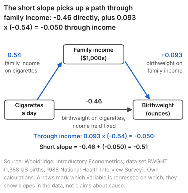
At 20 cigarettes a day the short model predicts a birthweight 10.28 ounces lower than at none, and the long model 9.27 ounces lower at the same family income. That is about 291 and 263 grams (28.35 grams to the ounce). Both compare mothers; neither predicts what giving up smoking would do.
The same reasoning accounts for the schooling coefficient. In these 526 workers experience and tenure both have positive coefficients in the long regression and are negatively correlated with schooling (-0.300 and -0.056). Leaving them out therefore pulled the schooling coefficient down, from 0.0920 to 0.0827. Experience accounts for about two thirds of that gap of 0.0093, tenure for about a third.
7. A simulation: more data, the same bias
A simulation checks the formula where the parameters are known, and shows what a larger sample does. \(X_1\) is standard normal and \(X_2 = 0.6X_1 + V\), with \(V \sim N(0, 0.64)\) (standard deviation 0.8) independent of \(X_1\), so \(X_2\) has variance \(0.36 + 0.64 = 1\) and slope \(\delta_1 = 0.6\) on \(X_1\). The outcome is \(Y = 1 + 0.5X_1 + 0.8X_2 + e\), with \(e \sim N(0, 1)\) independent of both: a long model satisfying the assumption, with \(\beta_1 = 0.5\) and \(\beta_2 = 0.8\). The short slope (\(Y\) on \(X_1\) alone) should be centred on \(0.5 + 0.8 \times 0.6 = 0.98\), the long slope on 0.5. We drew 10,000 samples at each of \(n = 50\), 200 and 2,000.
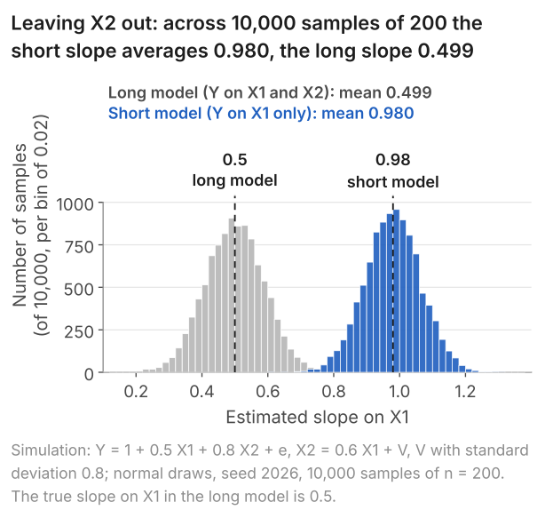
The table gives the means and standard deviations of the two slopes at all three sample sizes.
| n | Short slope: mean | Short slope: SD | Long slope: mean | Long slope: SD |
|---|---|---|---|---|
| 50 | 0.9786 | 0.1721 | 0.4980 | 0.1832 |
| 200 | 0.9795 | 0.0845 | 0.4992 | 0.0893 |
| 2,000 | 0.9798 | 0.0268 | 0.4995 | 0.0280 |
The short slope's mean stays at 0.98 while its standard deviation falls from 0.172 to 0.027, a factor of 6.4 in these samples, close to the \(\sqrt{2000/50} = 6.3\) of lesson 5's rule. The distribution narrows around the wrong value (Figure 3). At \(n = 50\), 21 of the 10,000 short slopes fall below 0.5; at 200 and 2,000, none does. All six means sit a little below their targets, each by less than two Monte Carlo standard errors (the standard deviation divided by 100, the square root of 10,000). That is chance; the seed was not changed.
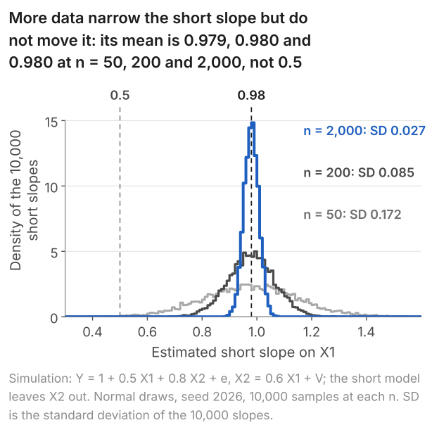
So the bias does not shrink with the sample size: the short-model estimator settles on \(\beta_1 + \beta_2\delta_1\), here 0.98, not on \(\beta_1\), and more data make it more precise about the wrong value. An estimator that settles on its parameter as \(n\) grows is called consistent; this one is biased and inconsistent for \(\beta_1\). Its standard errors give no warning: at \(n = 200\) they average 0.0845, the standard deviation of the 10,000 short slopes, so they measure the spread and say nothing about the centre. The same holds for the births. More births would narrow lesson 11's interval for the short slope, -0.691 to -0.336, but, if the long model holds, around \(\beta_1 + \beta_2\delta_1\), whose second term this sample estimates at \(\hat\beta_2\tilde\delta_1 = -0.050\).
8. Including a variable that does not belong
The opposite mistake, putting in a regressor whose coefficient is zero, costs precision rather than bias. In a second simulation \(Y = 1 + 0.5X_1 + e\) and \(X_3 = 0.5X_1 + W\), with \(W \sim N(0, 0.75)\) (standard deviation 0.87), so \(X_3\) has variance 1, correlation 0.5 with \(X_1\) and coefficient zero. In 10,000 samples of 200 we fitted \(Y\) on \(X_1\), with and without \(X_3\).
The regression with \(X_3\) is a long model satisfying the assumption, so including \(X_3\) brings no bias. It does cost precision. With \(X_3\) in the regression, the \(X_1\) coefficient is the slope on the part of \(X_1\) that \(X_3\) does not predict (lesson 12). At a correlation of 0.5, \(X_3\) predicts a quarter of the variance of \(X_1\) (\(0.5^2 = 0.25\)). A slope estimated from less variation in its regressor is less precise (lesson 11): in large samples its variance rises by the factor \(1/0.75\), and its standard deviation by \(1/\sqrt{0.75} = 1.155\), or 15.5%. The table gives the simulated slopes.
| Regression | Mean of the \(X_1\) slope | SD of the \(X_1\) slope |
|---|---|---|
| \(X_3\) left out | 0.4998 | 0.0714 |
| \(X_3\) included | 0.4993 | 0.0826 |
Both means are close to 0.5, and the \(X_3\) coefficient's estimates average 0.0010. The standard deviation of the \(X_1\) slope rises by 15.7% in these samples, from 0.0714 to 0.0826, close to the 15.5% expected. A zero-coefficient variable uncorrelated with \(X_1\) would leave the standard deviation where it was; overlapping regressors in general are lesson 16's subject (course home).
A sample cannot show that a coefficient is zero in the population, though its estimate can be close to zero. In the 526 workers, adding nonwhite (1 for a non-white worker, 0 otherwise) to the regression of log wage on schooling gives it a coefficient of -0.0042, with t = -0.06 and a 95% interval of -0.140 to 0.132. The schooling coefficient moves from 0.08274 to 0.08271.
9. Variables we cannot measure
When the left-out variable is not in the data, neither factor of the product can be estimated, and the sign rule becomes a prediction. The standard case is ability in a wage equation. The regression of log wage on schooling for the 526 workers does not hold ability fixed, because WAGE1 does not measure it: ability sits in the error with everything else the regression leaves out. It is likely that more able people earn more than others with the same schooling. They are also likely to have more schooling. Hence we expect \(\beta_2 > 0\) and \(\delta_1 > 0\), and, if a long model with ability in it holds, an upward bias in the schooling coefficient of the regression without ability.
That direction is a prediction from two signs, not a calculation. The left-out variables we could add, experience and tenure, pulled the schooling coefficient down (0.0920 with them, 0.0827 without); the one we cannot add is expected to pull it up. So neither 0.083 nor 0.092 is "the effect of education". Each compares workers, the second with experience and tenure held fixed, and both leave ability in the error. The page on correlation and causation takes this further.
Left-out variables are one reason the assumption fails. Measurement error in a regressor and simultaneity, where the outcome also moves the regressor, are two others; the instrumental variables page sets them out side by side.
10. What can be done
What can be done depends on whether the left-out variable is in the data. If it is, add it: including a variable as a regressor is what "controlling for" it means (lesson 12). Whether a control belongs depends on the two conditions of section 4, not on its t-statistic. A control with a small t can still have a non-zero coefficient, and dropping it then biases any regressor it moves with.
A control takes one variable out of the error and leaves the rest in it. With income in the birthweight regression, the mother's education, health and care in pregnancy remain in the error. In the 1,387 births with the mother's schooling recorded, her schooling is lower among heavier smokers, by 0.085 years per cigarette a day. It is likely that some of these factors go with heavier babies and with less smoking. If so, a downward bias may remain even with income held fixed. The mother's schooling is in these data and can be added as a control; her health and care in pregnancy need better data, such as a record of her visits to a doctor.
When the variable cannot be measured, as with ability, an instrument may help. An instrument is a variable that moves with the regressor but is uncorrelated with the error, so that it has no part in the outcome except through the regressor. A control goes into the regression, to take a variable out of the error; an instrument stays out, and picks out the part of the regressor's variation that is unrelated to the error. The instrumental variables page sets out the estimator, and lesson 20 will teach it (course home).
When the regressor is a 0/1 treatment, the same problem is called selection bias. If those who take the treatment differ from those who do not in ways that also move the outcome, the treatment dummy is correlated with the error (lesson 17, course home). And with several regressors in both models, the slope of the left-out variable in the identity is a partial one, given the other included regressors, so a sign predicted from simple correlations can be wrong.
11. Common mistakes
- "Leaving out a variable that matters biases the other coefficients." Only if it is also correlated with them. In the simulation cell with \(\beta_2 = 0.8\) and \(\delta_1 = 0\), the short slope averaged 0.4994, against 0.5.
- "The gap between the short and the long coefficient is the bias." The -0.050 for the births is a fact about this sample. The bias is a property of the estimator across samples, and needs the long model to hold.
- "A large enough sample removes the bias." At \(n = 2{,}000\) the short slope averaged 0.980, with a standard deviation of 0.027, against \(\beta_1 = 0.5\).
- "The short coefficient is too low, so it understates the link between smoking and birthweight." -0.514 is below -0.463, and if the long model holds the bias is downwards. For a negative coefficient that means the short regression overstates how much smoking goes with lower birthweight.
- "Adding every available variable is the safe choice." A variable with coefficient zero and correlation 0.5 with \(X_1\) raised the standard deviation of the \(X_1\) slope by 15.7% in the simulation.
- "The long regression's coefficient is the effect." Only if its error satisfies the assumption. Ability is still in the error of the wage regression, and the mother's education in that of the births.
12. Check your understanding
Five questions, marked on the page; every option has an explanation, including the wrong ones. (Without JavaScript the explanations are shown beneath each question.)
1. A regression of house prices on floor area leaves out distance from the city centre. Suppose that, at the same floor area, distance goes with lower prices (\(\beta_2 < 0\)), and that larger houses lie farther from the centre (\(\delta_1 > 0\)). If the long model holds, which way is the short-model estimator of the floor-area coefficient biased?
This uses one of the two signs, \(\delta_1 > 0\). The bias is \(\beta_2\) times \(\delta_1\), and \(\beta_2\) is negative here, so the product is negative: the positive correlation on its own does not set the direction.
The two signs multiply; they do not add. A negative times a positive is negative, so the bias is downwards. The bias is zero only when one of the two factors is zero.
Correct. The sign of the bias is the sign of \(\beta_2\) times the sign of \(\delta_1\): negative times positive is negative, so the short-model estimator is centred below the long model's floor-area coefficient. This is the cell of the sign table that WAGE1 and the birthweight data leave empty; with \(\beta_2 = -0.8\) and \(\delta_1 = 0.6\) the bias would be \(-0.48\).
2. A long model \(Y = \beta_0 + \beta_1 X_1 + \beta_2 X_2 + u\) satisfies its assumption, with \(\beta_2 = -0.5\), and the population slope of \(X_2\) on \(X_1\) is \(\delta_1 = 0.4\). A regression leaves \(X_2\) out. What is the bias of the short-model estimator of \(\beta_1\) in large samples?
Correct. The bias is \(\beta_2\) times \(\delta_1\): \(-0.5 \times 0.4 = -0.20\). The short-model estimator settles on \(\beta_1 - 0.20\), below \(\beta_1\).
This adds the two factors, \(-0.5 + 0.4 = -0.10\). The bias is their product, \(-0.20\): the left-out variable's coefficient scaled by how far \(X_2\) moves per unit of \(X_1\).
This has the right size and the wrong sign. Leaving a variable out does not push a coefficient up as a rule: here \(\beta_2\) is negative and \(\delta_1\) positive, so the product is \(-0.20\), a downward bias.
This is \(\delta_1\) alone. The slope of \(X_2\) on \(X_1\) says how far \(X_2\) moves with \(X_1\); it biases the coefficient only through \(\beta_2\), which scales it: \(-0.5 \times 0.4 = -0.20\).
3. In the 1,388 births, adding male (1 for a boy, 0 for a girl) to the regression of birthweight on cigarettes a day gives male a coefficient of 2.94 ounces (t = 2.7) and moves the cigarette coefficient from -0.5138 to -0.5137. The slope of male on cigarettes is zero to four decimals. Which condition for omitted variable bias fails here?
Male has a coefficient of 2.94 ounces with t = 2.7: in these births, boys are on average 2.94 ounces heavier than girls born to mothers who smoke the same amount. That condition holds; it is the other one that fails.
Correct. The slope of male on cigarettes is zero to four decimals, so the product of the two factors is about zero and the cigarette coefficient moves by 0.0001. Bias needs a non-zero coefficient and a correlation with the regressor; here the second fails.
Male matters for birthweight, which is one condition. The other, a correlation with cigarettes, fails: the slope of male on cigarettes is zero to four decimals, and leaving male out moves the cigarette coefficient by only 0.0001.
4. For the 1,388 births, the cigarette coefficient is -0.5138 without family income and -0.4634 with it. The gap, -0.0504, equals \(0.0928 \times (-0.5429)\): the income coefficient in the long regression times the slope of income on cigarettes. Which statement about the -0.0504 is right?
Correct. Short = long + (coefficient on income) times (slope of income on cigarettes) is algebra about two least-squares fits on the same data: \(-0.4634 + 0.0928 \times (-0.5429) = -0.5138\). It holds in every sample, whatever the population model, and by itself says nothing about bias.
The bias is a property of the estimator across repeated samples, \(\beta_2\delta_1\), and is defined under a long model whose error satisfies the assumption. -0.0504 is a fact about this one sample; if the long model holds it estimates the bias, but it is not the bias.
With more births, if the long model holds, the two factors would settle on \(\beta_2\) and \(\delta_1\), so the gap would settle on their product, not on zero, unless one of them is zero. In the simulation of section 7 the gap between the mean short and long slopes stayed at 0.48 at all three sample sizes.
5. In the simulation of section 7, \(Y = 1 + 0.5X_1 + 0.8X_2 + e\) and \(X_2 = 0.6X_1 + V\). At \(n = 50\) the short slope (\(Y\) on \(X_1\) alone) averaged 0.9786 over 10,000 samples. Around what value is the short slope centred at \(n = 2{,}000\)?
0.5 is \(\beta_1\), the centre of the long slope. The short slope is centred on \(\beta_1 + \beta_2\delta_1 = 0.5 + 0.8 \times 0.6 = 0.98\) at every sample size: more data narrow it around 0.98; they do not move it to 0.5.
This shrinks the bias of 0.48 as a standard error shrinks, by \(\sqrt{2000/50} = 6.3\): \(0.5 + 0.48/6.3 = 0.58\). The standard deviation does fall that way (0.172 to 0.027), but the centre does not move: the bias does not depend on \(n\).
Correct. The short slope is centred on \(\beta_1 + \beta_2\delta_1 = 0.5 + 0.8 \times 0.6 = 0.98\) whatever \(n\) is. In these samples it averaged 0.9798 at \(n = 2{,}000\), with a standard deviation of 0.0268: more precise, about the same wrong value.
This adds the whole of \(\beta_2\) to \(\beta_1\): \(0.5 + 0.8 = 1.3\). The short slope picks up \(\beta_2\) only in proportion to how far \(X_2\) moves with \(X_1\), \(\delta_1 = 0.6\): \(0.8 \times 0.6 = 0.48\), so the centre is 0.98.
13. Three questions about omitted variable bias
Omitted variable bias is the gap between a coefficient's average across samples and its parameter when a left-out variable matters for the outcome and is correlated with the regressor. It equals the left-out variable's coefficient times its slope on the regressor. In 1,388 US births (1988), leaving income out moves the cigarette coefficient from -0.463 to -0.514, estimating that product.
Multiply two signs: the left-out variable's coefficient in the full model and its correlation with the included regressor. A positive product biases the coefficient upwards, a negative one downwards. In 1,388 US births (1988), higher income goes with heavier babies and smokers have lower incomes, so leaving income out biases the cigarette coefficient downwards, if the model with income holds.
No. The estimator from the regression without the variable settles on the wrong value as the sample grows: more data narrow its distribution but do not move its centre. In a simulation with a slope of 0.5, that regression's slope averaged 0.979, 0.980 and 0.980 in 10,000 samples of 50, 200 and 2,000.
14. Where next
- Lesson 14: dummies, logs, elasticities and interactions, which puts groups, percentages and slopes that differ between groups into a regression.
- Lesson 12: multiple regression and holding other things fixed, for what a coefficient means when other regressors are in the model.
- Instrumental variables and weak instruments, for what to do when the left-out variable cannot be measured.
- Correlation versus causation, for why a comparison between groups is not an effect.
- The course home, which lists all 25 lessons and says which are published.
Stuck on an omitted variable question? Send it
I tutor statistics and econometrics one-to-one, from a first regression through to instruments, panel data and time series. Bring the question you are stuck on and we will work through it in the free 30-minute consultation.
Book a free 30-minute consultation Econometrics tutor: how it works
Data and simulation. Birthweights: Wooldridge, Introductory Econometrics: A Modern Approach, data set BWGHT (1,388 births, 1988 National Health Interview Survey); results quoted, data not republished. Wages: Wooldridge, Introductory Econometrics: A Modern Approach, data set WAGE1 (526 US workers, 1976 Current Population Survey); results quoted, data not republished. Simulation of section 7 (Figures 2 and 3): for each sample size (50, 200, 2,000) a fresh numpy default_rng(2026); X1, V and e drawn in that order as three calls of rng.standard_normal((10000, n)), each row one sample; X2 = 0.6 * X1 + 0.8 * V (so the scaled noise has variance 0.64) and Y = 1 + 0.5 * X1 + 0.8 * X2 + e; the short slope from Y on a constant and X1, the long slope from Y on a constant, X1 and X2, both by least squares. Table of section 5: a fresh default_rng(2026) for each cell, the same three calls with n = 200, X2 = delta1 * X1 + sqrt(1 - delta1**2) * V and Y = 1 + 0.5 * X1 + beta2 * X2 + e; the cell with 0.8 and 0.6 is the n = 200 run of section 7. Section 8: a fresh default_rng(2026); X1, W and e drawn in that order as three calls of rng.standard_normal((10000, 200)); X3 = 0.5 * X1 + sqrt(0.75) * W (so the scaled noise has variance 0.75) and Y = 1 + 0.5 * X1 + e. Adapted from my lecture notes for Econometric Methods (ECON61001, Section B, 2014 to 2016), the MSc pre-sessional statistics course (ECON60901, 2015) and Cross-Section Econometrics (ECON60052, 2019) at the University of Manchester.