
Among 526 US workers in 1976, a year more schooling goes with about 8.3% higher pay. But the better-educated also average less experience, so the 8.3% compares workers who differ in both. A regression with several regressors gives each a coefficient: the predicted difference between workers one unit apart in it and alike in the others. That is multiple regression.
In this lesson
- Why one regressor is not enough
- The model with several regressors
- What holding other things fixed means
- How the coefficients are found
- Reading the table: 526 workers
- Partialling out: how the others are held fixed
- What adding a regressor does to the others
- What reading a coefficient as an effect needs
- Common mistakes
- Check your understanding: five marked questions
- Three questions about multiple regression
- Where next
1. Why one regressor is not enough
A regression with one regressor makes one comparison, and that comparison can mix several differences at once. Lesson 9 fitted pay on schooling for five made-up workers. The OLS explainer, in its second example, fits the logarithm of the hourly wage on years of education for 526 real ones, US workers surveyed in 1976 (Wooldridge's WAGE1 data), and the slope is 0.0827. ("Log" on this page always means the natural logarithm.) Read as 100 times the coefficient, one more year of schooling goes with about 8.3% higher hourly pay in these workers.
But in these 526 workers, those with more education have less potential experience, the years in which they could have been at work: the correlation between the two is -0.300. So workers one year apart in schooling also differ, on average, in experience. If experience goes with pay too, the 8.3% contains some of that association, and a regression with schooling as its only regressor cannot separate the two. A regression with both as regressors gives each its own coefficient.
What students say
“Nicky is an excellent econometrics tutor. He explains complex concepts clearly and makes them much easier to understand.”
“I was completely lost in my economics class, and then I started working Nicky and he totally saved me. He was excellent at explaining the material and extremely accommodating to meet with me many times despite us being in different time zones! Highly recommend working with Nicky!”
“Nicky is a very good and thorough teacher. He has excellent knowledge of econometrics and takes the time to work through your questions. Highly recommended!”
“Really great tutor! Encouraging, knowledgeable, friendly”
“Very good lesson, Nicky is very helpful.”
“Very helpful and clear.”
“I gather it was very useful, thank you!”
“Fantastic!”
2. The model with several regressors
The multiple regression model writes the dependent variable as an intercept, plus one term for each regressor, plus an error. For the workers, with three regressors:
$$ \begin{aligned} \ln(\text{wage}_i) &= \beta_0 + \beta_1\,\text{educ}_i \\ &\quad + \beta_2\,\text{exper}_i + \beta_3\,\text{tenure}_i \\ &\quad + u_i , \end{aligned} $$where educ is years of education, exper years of potential experience and tenure years with the current employer. The coefficients \(\beta_0, \dots, \beta_3\) are fixed numbers describing the population the 526 workers were drawn from; we do not know them, and the regression estimates them. The error \(u_i\) is everything else that goes into worker \(i\)'s log wage, measured or not, such as ability, effort and luck: the part generated over and above the regressors.
Definition: the multiple regression model
With \(k\) regressors, the model for individual \(i\) is
$$ \begin{aligned} Y_i = \beta_0 &+ \beta_1 X_{1i} + \beta_2 X_{2i} \\ &+ \dots + \beta_k X_{ki} + u_i , \end{aligned} $$for \(i = 1, \dots, n\). \(Y_i\) is the dependent variable; \(X_{1i}, \dots, X_{ki}\) are the regressors (the first subscript names the regressor, the second the individual); \(\beta_0\) is the intercept and \(\beta_1, \dots, \beta_k\) the slope coefficients; \(u_i\) is the error. With \(k\) regressors there are \(k + 1\) coefficients: four in the wage model, where \(k = 3\).
Remarks. Suppose the error averages zero whatever the values of the regressors, the assumption that section 8 examines. Then the average value of \(Y\) for individuals with particular values \(x_1, \dots, x_k\) of the regressors is \(\beta_0 + \beta_1 x_1 + \dots + \beta_k x_k\). Hence \(\beta_j\) is the difference in that average between two groups whose values of \(X_j\) differ by one and whose other regressors in the model are equal. The model holds fixed only the regressors in it. Ability is not in WAGE1, so it is part of \(u_i\), and two workers with the same schooling, experience and tenure can differ in it.
On the letters: a capital, as in \(Y_i\) and \(X_{ji}\), marks a variable treated as random, whose value is not known until individual \(i\) is drawn; the lower-case \(y_i\) and \(x_{ji}\) are the values in hand, the numbers in the data file. Lesson 11 wrote the simple model with the data in lower case, \(y_i = \beta_0 + \beta_1 x_i + u_i\). The error \(u_i\) is random too, and keeps the lower-case letter that every earlier page gives it. Books use other letters (Wooldridge writes \(x\) and \(u\) in lower case; others write \(\varepsilon\) for the error), and the choice is cosmetic.
3. What holding other things fixed means
"Holding other things fixed" describes a comparison between observations, made with the fitted equation. Least squares, extended to several regressors in section 4, gives this fitted equation for the 526 workers:
$$ \begin{aligned} \widehat{\ln(\text{wage})} &= 0.2844 + 0.0920\,\text{educ} \\ &\quad + 0.0041\,\text{exper} \\ &\quad + 0.0221\,\text{tenure} . \end{aligned} $$The hat marks a predicted value. Take two workers with the same experience and tenure, one year apart in schooling, and work out both predictions. The table does it at two settings.
| Experience (years) | Tenure (years) | Predicted log wage, 12 years of schooling | Predicted log wage, 13 years | Gap |
|---|---|---|---|---|
| 5 | 2 | 1.453 | 1.545 | 0.092 |
| 20 | 5 | 1.581 | 1.673 | 0.092 |
For the first worker in the table the prediction is 0.2844 + 0.0920 × 12 + 0.0041 × 5 + 0.0221 × 2 = 1.453. Within a pair the experience and tenure terms are the same for both workers, so only the schooling term differs, by 0.0920 × 1. Hence the gap is 0.092 in both rows: the coefficient on educ. A difference in log wage is measured in log points, and 0.092 log points is about 9.2% higher predicted pay.
That the gap is the same in both rows is an assumption of the model, not a finding: the equation has no term that lets the schooling gap depend on experience or tenure. Lesson 14 adds such a term. Nor does the equation need workers at each setting: 97 of the 526 are within two years of the first setting in both experience and tenure, and only 18 of the second.
This is the reading of every coefficient in a multiple regression: the difference in predicted \(Y\) between two observations that differ by one unit in that regressor and have the same values of every other regressor in the model. For educ: comparing workers with the same experience and tenure, one more year of schooling goes with a predicted log wage 0.092 higher. "Controlling for experience" means including experience as a regressor, so that the other coefficients compare workers with the same experience. "Ceteris paribus", Latin for "other things equal", is the name books give to the same comparison.
The comparison is not an experiment. Nobody's schooling was raised while their experience was held at 5 years: the 526 workers were surveyed as they were. The regression holds fixed only what is in it, and the two workers of a pair may differ in ability. So the coefficient is an association. Reading it as the effect of one more year of schooling needs the assumption that nothing left in the error moves with the regressors.
4. How the coefficients are found
Least squares chooses the \(k + 1\) coefficients by the rule that lesson 9 used for an intercept and one slope. For trial values \(b_0, b_1, \dots, b_k\), each observation has a gap between its \(y_i\) and the trial prediction. Square the gaps and add them up:
$$ \begin{aligned} &S(b_0, b_1, \dots, b_k) \\ &= \sum_{i=1}^{n} \big(y_i - b_0 - b_1 x_{1i} \\ &\qquad - \dots - b_k x_{ki}\big)^2 . \end{aligned} $$In words: S is the sum, over all observations, of the squared gap between the observed value and the trial prediction.
The data are fixed here; only the trial values vary. The estimates \(\hat\beta_0, \dots, \hat\beta_k\) are the trial values that make \(S\) smallest. In essence, least squares chooses the coefficients that make the fitted values as close as possible to the observed \(y_i\). \(S\) is in squared units of \(Y\): log points squared for the wages.
At the minimum the derivative of \(S\) with respect to each trial value is zero: \(k + 1\) equations in \(k + 1\) unknowns. With one regressor they solve by hand to lesson 9's formula. With several there is no formula as short as lesson 9's: already with two, the formula for one slope involves the variances and the covariance of both. In general the solution is written in matrix form, as on the OLS derivation page, and computed by software. It is unique provided no regressor is an exact linear combination of a constant and the others, as it would be if the same regressor were included twice; lesson 14 meets the standard example, the dummy variable trap.
The same equations give two facts about the residuals \(\hat u_i = y_i - \hat y_i\), which are not the errors \(u_i\) (lesson 10 keeps the two apart). Provided the regression has an intercept, in every sample:
- The residuals sum to zero, so they average zero.
- The residuals are uncorrelated with every regressor. For each regressor, the sample correlation between it and the residuals is zero.
Show where the two facts come from
- The intercept's equation. The derivative of \(S\) with respect to \(b_0\) is -2 times the sum of the gaps. At the least-squares values each gap is a residual, so \(-2\sum_i \hat u_i = 0\): the residuals sum to zero.
- Each slope's equation. The derivative with respect to \(b_j\) is -2 times the sum of \(x_{ji}\) times the gap, so \(\sum_i x_{ji}\,\hat u_i = 0\) for \(j = 1, \dots, k\).
- From sums to correlations. The numerator of the sample covariance between \(x_j\) and the residuals is $$ \begin{aligned} &\textstyle\sum_i (x_{ji} - \bar x_j)\,\hat u_i \\ &= \textstyle\sum_i x_{ji}\hat u_i - \bar x_j \sum_i \hat u_i , \end{aligned} $$ and both sums are zero by steps 1 and 2. So the covariance is zero, and so is the correlation.
Partialling out, in section 6, rests on the second fact.
5. Reading the table
A multiple-regression table has one row for each coefficient, and each row is read with the holding-fixed sentence of section 3. Here is the regression of log wage on schooling, experience and tenure for the 526 workers.
| Variable | Coefficient | Std. error | t | p-value | 95% interval |
|---|---|---|---|---|---|
| educ | 0.0920 | 0.0073 | 12.56 | 0.000 | 0.0776 to 0.1064 |
| exper | 0.0041 | 0.0017 | 2.39 | 0.017 | 0.0007 to 0.0075 |
| tenure | 0.0221 | 0.0031 | 7.13 | 0.000 | 0.0160 to 0.0281 |
| constant | 0.2844 | 0.1042 | 2.73 | 0.007 | 0.0797 to 0.4890 |
The whole regression: n = 526, R-squared = 0.316, adjusted R-squared = 0.312, root MSE = 0.441. A p-value printed as 0.000 is below 0.0005, not zero.
The same results as R and Python print them, with the commands that produce them:
R: the code
library(wooldridge)
data("wage1")
fit <- lm(lwage ~ educ + exper + tenure, data = wage1)
summary(fit)
confint(fit)
R: what it prints
> library(wooldridge)
> data("wage1")
> fit <- lm(lwage ~ educ + exper + tenure, data = wage1)
> summary(fit)

Call:
lm(formula = lwage ~ educ + exper + tenure, data = wage1)

Residuals:
     Min       1Q   Median       3Q      Max
-2.05802 -0.29645 -0.03265  0.28788  1.42809

Coefficients:
            Estimate Std. Error t value Pr(>|t|)
(Intercept) 0.284360   0.104190   2.729  0.00656 **
educ        0.092029   0.007330  12.555  < 2e-16 ***
exper       0.004121   0.001723   2.391  0.01714 *
tenure      0.022067   0.003094   7.133 3.29e-12 ***
---
Signif. codes:  0 ‘***’ 0.001 ‘**’ 0.01 ‘*’ 0.05 ‘.’ 0.1 ‘ ’ 1

Residual standard error: 0.4409 on 522 degrees of freedom
Multiple R-squared:  0.316,	Adjusted R-squared:  0.3121
F-statistic: 80.39 on 3 and 522 DF,  p-value: < 2.2e-16

> confint(fit)
                   2.5 %     97.5 %
(Intercept) 0.0796755675 0.48904351
educ        0.0776292151 0.10642876
exper       0.0007356984 0.00750652
tenure      0.0159896854 0.02814475
Python: the code
import wooldridge
import statsmodels.formula.api as smf

wage1 = wooldridge.data("wage1")
fit = smf.ols("lwage ~ educ + exper + tenure", data=wage1).fit()
print(fit.summary())
Python: what it prints
                            OLS Regression Results
==============================================================================
Dep. Variable:                  lwage   R-squared:                       0.316
Model:                            OLS   Adj. R-squared:                  0.312
Method:                 Least Squares   F-statistic:                     80.39
Date:                Thu, 08 Oct 2026   Prob (F-statistic):           9.13e-43
Time:                        14:49:41   Log-Likelihood:                -313.55
No. Observations:                 526   AIC:                             635.1
Df Residuals:                     522   BIC:                             652.2
Df Model:                           3
Covariance Type:            nonrobust
==============================================================================
                 coef    std err          t      P>|t|      [0.025      0.975]
------------------------------------------------------------------------------
Intercept      0.2844      0.104      2.729      0.007       0.080       0.489
educ           0.0920      0.007     12.555      0.000       0.078       0.106
exper          0.0041      0.002      2.391      0.017       0.001       0.008
tenure         0.0221      0.003      7.133      0.000       0.016       0.028
==============================================================================
Omnibus:                       11.534   Durbin-Watson:                   1.769
Prob(Omnibus):                  0.003   Jarque-Bera (JB):               20.941
Skew:                           0.021   Prob(JB):                     2.84e-05
Kurtosis:                       3.977   Cond. No.                         135.
==============================================================================

Notes:
[1] Standard Errors assume that the covariance matrix of the errors is correctly specified.
Read the coefficients first, each with the others held fixed:
- educ, 0.0920. Comparing workers with the same experience and tenure, one more year of schooling goes with a predicted log wage 0.0920 higher: about 9.2% higher pay.
- exper, 0.0041. Comparing workers with the same schooling and tenure, one more year of potential experience goes with about 0.4% higher pay.
- tenure, 0.0221. Comparing workers with the same schooling and experience, one more year with the current employer goes with about 2.2% higher pay.
- constant, 0.2844. The predicted log wage at zero schooling, experience and tenure. No worker has zero experience (the smallest value is 1 year), so the constant is not read on its own.
Each slope is a difference in log wage per year, and 100 times it is approximately the percentage difference in pay: a percentage of pay, not dollars and not percentage points. For educ the exact figure is 9.6%, because a difference of 0.0920 in log pay multiplies predicted pay by \(e^{0.0920} = 1.096\). The gap between the two readings grows with the size of the coefficient, as the table in the logs explainer shows.
Then the standard errors, each read as in lesson 11: an estimate of the standard deviation of that coefficient across repeated samples of 526 workers. With several regressors the degrees of freedom are \(n - k - 1 = 526 - 3 - 1 = 522\), one fewer for each of the four coefficients, in place of lesson 11's \(n - 2\). For educ, t = 0.09203/0.00733 = 12.56, and the 95% interval is 0.09203 ± 1.965 × 0.00733, or 0.0776 to 0.1064 (1.965 is the two-sided 5% critical value of t on 522 degrees of freedom). The data are compatible with a schooling coefficient anywhere from about 7.8% to 10.6% a year, with experience and tenure held fixed.
Last, the fit. R-squared is 0.316, against 0.186 for log wage on schooling alone. Adding a regressor gives least squares one more coefficient to choose, and setting it to zero would reproduce the old fit. So the smallest value of \(S\), the residual sum of squares, cannot rise (here it fell from 120.77 to 101.46), and R-squared cannot fall, whatever the regressor; the R-squared explainer shows it with columns of random numbers. The rise is therefore not evidence that experience and tenure belong. Adjusted R-squared charges for each coefficient and can fall when one is added; here it rose too, from 0.184 to 0.312.
6. Partialling out: how the others are held fixed
Section 3's comparison was made with the fitted equation, not by finding pairs of workers with equal experience and tenure. This section shows how least squares makes it from the data: it takes out of schooling the part that experience and tenure predict, and uses what is left.
- Regress schooling on the other regressors. Fitting educ on a constant, exper and tenure gives: predicted educ = 13.575 - 0.0738 exper + 0.0477 tenure, with R-squared 0.101.
- Keep the residual. For each worker, \(\hat r_{1i}\) is educ minus predicted educ: the part of schooling that experience and tenure do not predict. A worker with \(\hat r_{1i} = 2\) has two years more schooling than the equation predicts for that experience and tenure. By the two facts of section 4, \(\hat r_1\) averages zero and is uncorrelated with exper and with tenure (both sample correlations are below \(2 \times 10^{-15}\) in size: zero up to rounding error).
- Regress log wage on the residual. The slope is 0.092029, and so is the coefficient on educ in the regression of section 5: the two agree to fifteen decimal places.
Figure 1 sets the simple slope beside the slope after experience and tenure are taken out. Its lower panel also takes them out of log wage, plotting the residual of log wage on exper and tenure against \(\hat r_1\). The part of log wage removed is a straight-line combination of experience and tenure, with which \(\hat r_1\) is uncorrelated, so the slope is the same as in step 3.
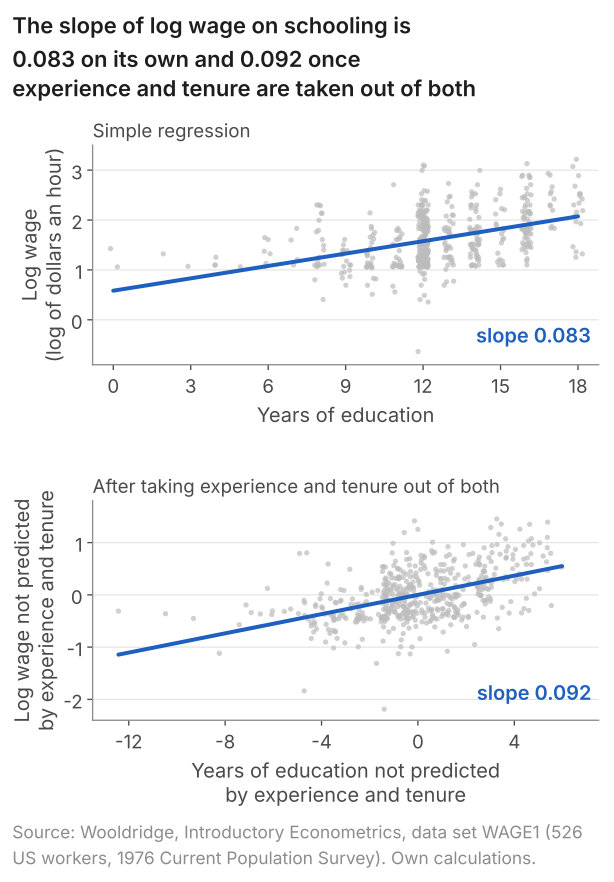
Because \(\hat r_1\) is uncorrelated with experience and tenure, workers with high and low values of it do not differ in experience or tenure on a straight-line fit. A regression on \(\hat r_1\) therefore compares workers who differ in schooling relative to their experience and tenure: the comparison of section 3. In the data, then, "with experience and tenure held fixed" means that the coefficient uses only the variation in schooling that they do not predict, 89.9% of its variance in these workers. What is removed is a straight-line prediction, because the model enters experience and tenure as straight-line terms. The two slopes are equal in every sample, not only in these data.
Show why the two slopes are equal in every sample
Write \(x_1\) for educ, \(x_2\) for exper and \(x_3\) for tenure.
- The slope on the residual. \(\hat r_1\) averages zero, so the slope of \(y\) on it is \(\sum_i \hat r_{1i} y_i\) divided by \(\sum_i \hat r_{1i}^2\).
- Substitute the full fit. Each \(y_i\) is its fitted value from the three-regressor regression plus its residual: $$ \begin{aligned} y_i &= \hat\beta_0 + \hat\beta_1 x_{1i} + \hat\beta_2 x_{2i} \\ &\quad + \hat\beta_3 x_{3i} + \hat u_i . \end{aligned} $$ Multiply by \(\hat r_{1i}\) and add over the workers.
- Four sums vanish. \(\hat r_1\) is the residual of the regression of \(x_1\) on a constant, \(x_2\) and \(x_3\), so by section 4 it sums to zero and has a zero sum of products with \(x_2\) and with \(x_3\). That removes the \(\hat\beta_0\), \(\hat\beta_2\) and \(\hat\beta_3\) terms. And \(\hat r_1\) is \(x_1\) minus a constant and multiples of \(x_2\) and \(x_3\), with each of which the residuals \(\hat u\) of the full regression have a zero sum of products, so \(\sum_i \hat r_{1i}\hat u_i = 0\).
- One sum is left. \(x_{1i}\) is its predicted value from step 1 of the section plus \(\hat r_{1i}\), and that predicted value is a constant plus multiples of \(x_2\) and \(x_3\). So \(\sum_i \hat r_{1i} x_{1i} = \sum_i \hat r_{1i}^2\), hence \(\sum_i \hat r_{1i} y_i = \hat\beta_1 \sum_i \hat r_{1i}^2\), and the slope on the residual is \(\hat\beta_1\).
No step uses the wage data or any assumption about the population. Books call the result the Frisch-Waugh theorem.
The two-step route reproduces the coefficient but not its standard error (0.0079 against 0.0073), because the residuals of step 3 still hold the part of log wage that experience and tenure predict; quote the standard error from the full regression.
7. What adding a regressor does to the others
Adding experience and tenure moved the schooling coefficient from 0.0827 to 0.0920. This section says when such a move happens. Figure 2 shows that case and a second one, each coefficient with its 95% interval. The second is from the 1,388 US births (1988) of lesson 11's second printout: adding family income to the regression of birthweight on cigarettes a day moved the cigarette coefficient from -0.5138 to -0.4634 ounces per cigarette.
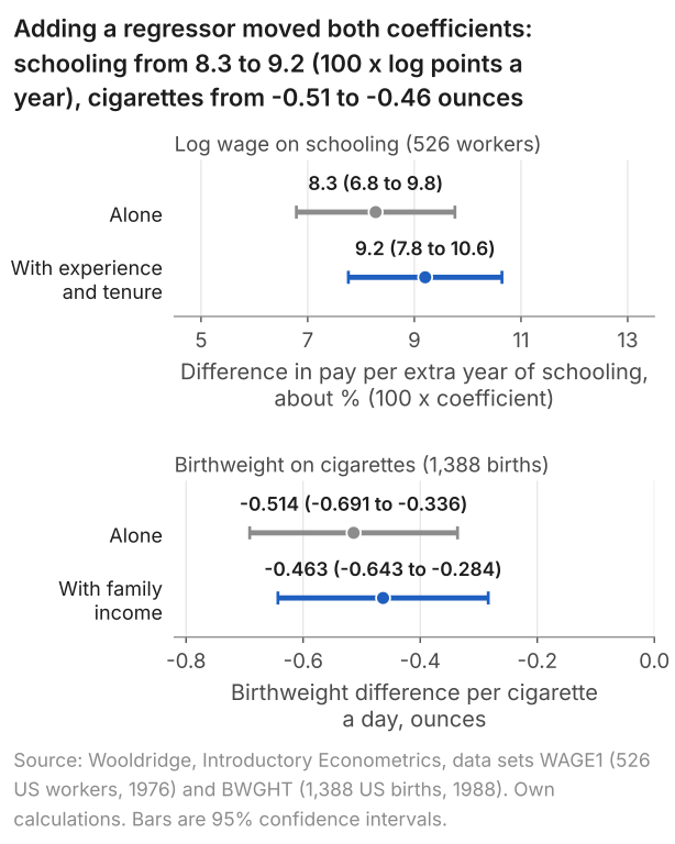
Start with what the short regression, log wage on schooling alone, compares. In these workers, one more year of schooling goes with 1.47 fewer years of potential experience on average (the correlation is -0.300). Experience goes with pay at given schooling and tenure: its coefficient in the longer regression is 0.0041. So workers one year apart in schooling also differ in experience, and the short regression's schooling coefficient picks up part of the association between experience and pay. Including experience controls for a factor that goes with pay and is correlated with schooling, and the schooling coefficient moves.
Hence a coefficient moves when a regressor is added only if two things hold together: the added regressor has a non-zero coefficient in the longer regression, and it is correlated with the regressor in question in the sample. If either fails, the coefficient stays exactly where it was. With no correlation there is no difference in the added regressor for the short coefficient to pick up; with a zero coefficient, that difference goes with no difference in the outcome. Both hold for experience. Tenure has the larger coefficient, 0.0221, but its correlation with schooling is only -0.056, and it accounts for about a third of the move. In the births, family income has a coefficient of 0.0928 ounces per 1,000 dollars and a correlation of -0.173 with cigarettes, so both hold there too. With other regressors already in the model, the correlation that counts is with the part of the regressor that they do not predict: the residual of section 6.
Which way a coefficient moves, and by how much, follows from the added regressor's coefficient in the longer regression times its slope on the regressor in question, net of the regressors the shorter regression already has. Lesson 13 works it out as an identity: exact algebra about two regressions on the same data, which needs no assumption. R-squared rose too (it cannot fall when a regressor is added), and that says nothing about which coefficients moved.
8. What reading a coefficient as an effect needs
Every reading so far has been a comparison. Reading a coefficient as an effect, such as the effect of one more year of schooling on pay, needs an assumption about the error, which holds everything the model leaves out. In words: given any values of the regressors, the error averages zero. In the course's plain words, nothing left in the error moves with the regressors. As a formula,
$$ \operatorname{E}[u_i \mid X_{1i}, \dots, X_{ki}] = 0 . $$In words: at every combination of the regressors' values, the average of the error is zero.
What it rules out is an error that moves with a regressor: in the wage equation, a part of pay left out of the model that is higher or lower on average for workers with more schooling, experience or tenure. A weaker statement, implied by it, is that the error is uncorrelated with each regressor: all the unobserved variables, and the variables we observe but have not included, are together uncorrelated with the regressors. For this lesson the difference does not matter. A regressor that satisfies the assumption is called exogenous. Under it, with random sampling and no regressor an exact combination of a constant and the others, the least-squares estimators are unbiased: centred on \(\beta_0, \dots, \beta_k\) across repeated samples. The Gauss-Markov page lists the full set of assumptions.
If the assumption holds for the wage model with schooling, experience and tenure, 0.092 is an estimate of the effect of one more year of schooling on log pay at given experience and tenure. The data cannot settle whether it holds: by section 4, the residuals are uncorrelated with the regressors in every sample, whether or not the errors are. In practice we must use economic reasoning to judge whether the assumption is likely to hold, and in the wage regression it is doubtful. Ability is in the error, and if it moves with schooling the assumption fails; lesson 13 shows what then happens to the coefficient.
A word of vocabulary: this is multiple regression, one dependent variable and several regressors. "Multivariate regression" means several dependent variables modelled together, and is not the name for the regressions of this lesson.
9. Common mistakes
- "The regression held experience fixed, as in an experiment." Nobody's experience was set. The coefficient compares surveyed workers with the same experience, through the fitted equation.
- "Held fixed means everything else is held fixed." Only the regressors in the model are. Ability is not in WAGE1, so two workers with the same schooling, experience and tenure can differ in it.
- "A coefficient is the same whatever else is in the regression." Schooling's is 0.0827 alone and 0.0920 with experience and tenure.
- "Any regressor that goes with the outcome moves the others when it is added." It must also be correlated with them; uncorrelated in the sample, it leaves them exactly where they were. Tenure's coefficient is larger than experience's (0.0221 against 0.0041), but its correlation with schooling is only -0.056, so it accounts for only about a third of the move.
- "R-squared rose, so the new regressors belong." R-squared cannot fall when a regressor is added, even a column of random numbers. The rise from 0.186 to 0.316 is a closer fit, not evidence that experience and tenure belong.
- "A coefficient of 0.0920 on log wage means 0.092 dollars, or 9.2 percentage points." It means about 9.2% higher pay per year of schooling: a percentage of pay.
10. Check your understanding
Five questions, marked on the page; every option has an explanation, including the wrong ones. (Without JavaScript the explanations are shown beneath each question.)
1. In these 526 workers (US, 1976), the regression of log wage on educ, exper and tenure gives tenure, years with the current employer, a coefficient of 0.0221. Which reading is right?
This reads the coefficient as the result of an intervention on one worker, as the phrase "held fixed" can suggest. The regression compares different workers in a 1976 survey; nobody's tenure was changed. Reading it as an effect needs the assumption that nothing left in the error moves with the regressors, and the reading is then conditional on that assumption.
Correct. A coefficient in a multiple regression is the difference in predicted log wage between two workers who differ by one unit in that regressor and have the same values of the other regressors in the model, here educ and exper. 100 × 0.0221 = 2.2, so about 2.2% higher pay per year of tenure.
It sounds like a plain reading of 2.2% per year, but it is the comparison a regression of log wage on tenure alone would make, and that regression gives 0.0240, about 2.4%. Workers with longer tenure also have more experience (the correlation between exper and tenure is 0.499 in these workers), so that comparison mixes the two. This coefficient compares workers with the same schooling and experience.
2. A report on 1,388 US births (1988) says: "controlling for family income, each extra cigarette a day goes with a birthweight 0.463 ounces lower". What was done with family income?
Correct. Controlling for a variable means including it as a regressor. The cigarette coefficient, -0.4634, then compares mothers one cigarette a day apart who have the same family income, through the fitted equation. All 1,388 births are used.
Comparing like with like sounds like what controlling means, but no birth is dropped: the regression uses all 1,388. It compares mothers with the same income through the fitted equation, by taking out of cigarettes the part that income predicts (partialling out). Exact matches on income are not needed.
Setting income equal for everyone sounds like holding it fixed. But if every mother had the same income, income would be a constant and could not be a regressor beside the intercept; the regression would be on cigarettes alone, with coefficient -0.5138, not -0.4634. The data are left as they are.
3. For these 526 workers the fitted equation is: predicted log wage = 0.2844 + 0.0920 educ + 0.0041 exper + 0.0221 tenure. Alone, schooling has a slope of 0.0827. Worker B has 3 more years of schooling and 2 more years of tenure than worker A, and the same experience. By how much does the fitted equation predict B's log wage to exceed A's?
This adds 0.0920 and 0.0221 once each. A coefficient is the predicted gap per unit of its regressor, so each is multiplied by the size of the difference: 3 years of schooling and 2 of tenure.
This counts the schooling difference only, 3 × 0.0920 = 0.276, as if being in the regression meant that differences in tenure did not count. Tenure is held fixed only between two workers with the same tenure; B has 2 more years, which adds 2 × 0.0221 = 0.0442.
This uses the simple slope for schooling: 3 × 0.0827 + 2 × 0.0221 = 0.292. In the fitted equation with experience and tenure the schooling coefficient is 0.0920, not 0.0827; the simple slope compares workers who also differ in experience and tenure.
Correct. Each coefficient is the predicted gap per unit of its regressor with the others held fixed, so the gaps add: 3 × 0.0920 + 2 × 0.0221 = 0.2760 + 0.0442 = 0.3202, about 0.320. Experience is the same for both workers, so its term cancels.
4. In 1,388 US births (1988), adding family income to the regression of birthweight on cigarettes a day moved the cigarette coefficient from -0.5138 to -0.4634. What has to be true of family income for such a move?
Income does go with birthweight, which makes this look enough, but not alone. If income were uncorrelated with cigarettes in the sample, mothers who smoke more would not differ in income on a straight-line fit, the short regression would have no income difference to pick up, and the coefficient would stay exactly at -0.5138.
The correlation is real (-0.173), which makes this look enough, but not alone. If income had a zero coefficient in the longer regression, differences in income would go with no difference in birthweight once cigarettes are in, and the cigarette coefficient would stay exactly at -0.5138, however strongly income moved with cigarettes.
Correct. Both are needed together, and both hold: income's coefficient in the longer regression is 0.0928 ounces per 1,000 dollars, and its correlation with cigarettes is -0.173. Lesson 13 shows how the two set the size of the move.
5. In a constructed data set of 200 observations, X2 has a sample correlation of exactly zero with X1. Adding X2 to the regression of Y on X1 gives X2 a coefficient of 0.30, with t = 6.1. What happens to the coefficient on X1?
X2 goes strongly with Y (0.30, with t = 6.1), which makes a change look certain. But a coefficient moves only if the added regressor has a non-zero coefficient and is also correlated with it in the sample, and the second does not hold here. With zero correlation, observations that differ in X1 do not differ in X2 on a straight-line fit, so there is nothing to pick up.
Correct. With zero sample correlation the second condition fails, so the coefficient on X1 is unchanged, exactly: this is algebra about two regressions on the same data. Its standard error can change, because the residuals change.
It can look as if a new regressor takes a share of what the old one explained, but an added regressor does not share out the existing coefficients. When a coefficient moves, it can move away from zero as well as towards it: in the wage data, schooling's rose from 0.0827 to 0.0920 when experience and tenure were added. Here it does not move at all.
11. Three questions about multiple regression
It means comparing observations with the same values of the other regressors in the model. In 526 US workers (1976), the schooling coefficient of 0.092 is the gap in predicted log wage between two workers one year apart in schooling with the same experience and tenure. Nothing is set by experiment, and variables left out are not held fixed.
A simple regression has one regressor; a multiple regression has several, and each coefficient compares observations alike in the others. In 526 US workers (1976), log wage on schooling alone gives a slope of 0.0827; adding experience and tenure gives 0.0920, where the second compares workers with the same experience and tenure.
It changes only if the added variable has a non-zero coefficient in the longer regression and is correlated in the sample with the regressor, net of the others already in the model. In 1,388 US births (1988), income's coefficient is 0.0928 ounces per 1,000 dollars and its correlation with cigarettes -0.173; adding it moved the coefficient from -0.514 to -0.463.
12. Where next
- Lesson 13: omitted variable bias: sign and size, which works out which way a coefficient moves when a regressor is left out, and by how much.
- Lesson 14: dummies, logs, elasticities and interactions, for 0/1 regressors and for a gap that differs between groups.
- How to read a regression table, the explainer, which reads every column of the printout of section 5.
- R-squared and adjusted R-squared, for what the fit statistics show and what they do not.
- The OLS estimator, derived, for least squares with several regressors in matrix form.
Stuck on a multiple regression question? Send it
I tutor statistics and econometrics one-to-one, from a first regression through to omitted variables, instruments and panel data. Bring the question you are stuck on and we will work through it in the free 30-minute consultation.
Book a free 30-minute consultation Econometrics tutor: how it works
Data. Wages: Wooldridge, Introductory Econometrics: A Modern Approach, data set WAGE1 (526 US workers, 1976 Current Population Survey); results quoted, data not republished. Birthweights: Wooldridge, Introductory Econometrics: A Modern Approach, data set BWGHT (1,388 births, 1988 National Health Interview Survey); results quoted, data not republished. One question uses a constructed data set, described in its stem. Adapted from my lecture notes for the MSc pre-sessional statistics course (ECON60901, 2015) and for Econometric Methods (ECON61001, Section B, 2014 to 2016) at the University of Manchester.