The Gauss-Markov theorem states that, under the classical linear model assumptions (linearity, exogeneity, homoskedasticity and no perfect multicollinearity), ordinary least squares is the Best Linear Unbiased Estimator: among all linear unbiased estimators of the coefficients, OLS has the smallest variance. Normality of the errors is not required.
How to read these notes
These notes are for a student who has met OLS and knows the regression model but wants to understand why OLS is the standard choice. The Gauss-Markov theorem is the formal justification, and it sits behind almost every introductory econometrics course. We focus on the meaning of each assumption and of the BLUE property, rather than the matrix algebra of the proof.
1. The classical linear regression model
Start with the linear model for a dependent variable \(y_i\) and regressors collected in the vector \(x_i\):
Here \(\beta\) is the vector of unknown coefficients we want to estimate and \(u_i\) is the error (or disturbance) term, capturing everything that affects \(y_i\) but is not in \(x_i\). OLS estimates \(\beta\) by choosing \(\hat\beta\) to minimise the sum of squared residuals \(\sum_i (y_i - x_i'\hat\beta)^2\). The question Gauss-Markov answers is: is this a good way to estimate \(\beta\), and in what sense?
2. The Gauss-Markov assumptions
The theorem holds under four conditions. They are the same assumptions you meet in the OLS notes, stated precisely.
The model is linear in the parameters: \(y_i = x_i'\beta + u_i\). The relationship can be non-linear in the variables (you can include \(x^2\), logs and interactions), but it must be linear in \(\beta\).
\(E[u_i \mid x_i] = 0\). The error has mean zero given the regressors, so the included variables carry no information about the unobserved component. This is the assumption that delivers unbiasedness, and the one that fails most often in practice.
\(\operatorname{Var}(u_i \mid x_i) = \sigma^2\) for every \(i\) (constant error variance), and the errors are uncorrelated across observations, \(\operatorname{Cov}(u_i, u_j)=0\) for \(i \neq j\). This is the assumption that delivers efficiency.
The regressors are not exact linear combinations of one another, so the design matrix has full rank. This simply guarantees that a unique OLS estimate exists.
Notice what is not on this list: there is no assumption that the errors are normally distributed. Normality is an extra ingredient used later for exact small-sample \(t\) and \(F\) tests, but it plays no role in the Gauss-Markov result itself.
3. Unbiasedness: getting it right on average
An estimator \(\hat\beta\) is unbiased if its expected value equals the true parameter, regardless of the sample we happen to draw:
Unbiasedness does not mean any single estimate equals \(\beta\) — sampling variation guarantees it will not. It means there is no systematic tendency to over- or under-shoot: if we could repeat the sampling many times and average the estimates, we would land on the truth. Under Assumptions 1, 2 and 4, OLS is unbiased. The exogeneity assumption \(E[u_i\mid x_i]=0\) is doing the work here; when it fails — through omitted variables, reverse causality or measurement error — OLS becomes biased and the rest of the theorem no longer matters.
4. Efficiency: the smallest variance
Being unbiased is not enough on its own. Many different estimators can be unbiased; we would like the one whose estimates are most tightly clustered around the truth — the one with the smallest variance. An unbiased estimator with the smallest variance in some class is called efficient.
A smaller sampling variance means narrower confidence intervals and more powerful hypothesis tests. Two unbiased estimators can both be "correct on average" while one is far more reliable in any given sample. Efficiency is about that reliability.
The standard normal density below is the reference distribution for an estimator's sampling variation. A more efficient estimator corresponds to a tighter, more peaked sampling distribution around \(\beta\).
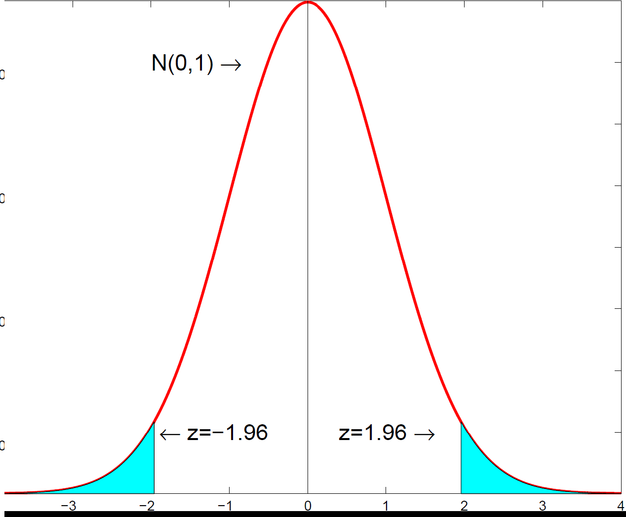 A more efficient estimator has a more concentrated sampling distribution around the true coefficient, giving sharper inference.
5. The theorem: OLS is BLUE
We can now state the result. Under Assumptions 1 to 4, ordinary least squares is the Best Linear Unbiased Estimator, usually abbreviated to BLUE. Each word is a restriction that, together, pins OLS down as the winner.
Best — smallest variance; Linear — the estimator is a linear function of the dependent variable \(y\); Unbiased — its expectation equals \(\beta\); Estimator. Among the whole class of estimators that are both linear in \(y\) and unbiased, none has a smaller variance than OLS.
Stated in terms of variances, for any other linear unbiased estimator \(\tilde\beta\),
This is a strong and reassuring statement. It says you cannot do better than OLS within the linear-unbiased class without bringing in extra information or extra assumptions. It is the reason OLS is the natural starting point in econometrics, and why so much of the subject is about checking whether its assumptions are credible.
"Linear" is a genuine restriction. There can exist non-linear or biased estimators with a smaller variance than OLS — Gauss-Markov does not rule those out. It only declares OLS best within the linear-unbiased family.
6. What happens when the assumptions fail
The value of the theorem is that it tells you exactly what you lose when a particular assumption breaks down.
- Exogeneity fails (\(E[u_i\mid x_i]\neq 0\)): OLS is biased and inconsistent. This is the serious case; the remedy is an identification strategy such as instrumental variables.
- Homoskedasticity fails (heteroskedasticity): OLS is still unbiased but no longer efficient, and the usual standard errors are wrong. The fix is heteroskedasticity-robust (White) standard errors.
- No autocorrelation fails (serial correlation, common in time series): again OLS is unbiased but not efficient, and standard errors need correcting.
In other words, losing efficiency is recoverable — you can patch the standard errors or use a more efficient estimator — but losing unbiasedness is not, and that is why exogeneity is the assumption econometricians worry about most. The practical machinery for detecting and handling these failures is covered in the notes on diagnostic testing.
7. Where normality comes in
If, in addition to the Gauss-Markov assumptions, we assume the errors are normally distributed, OLS becomes the best unbiased estimator — best now among all unbiased estimators, not just the linear ones — and the \(t\) and \(F\) statistics have exact \(t\) and \(F\) distributions in finite samples. Without normality, those distributions hold only approximately, justified in large samples by the central limit theorem. So normality is about the form of the sampling distribution used for inference, while Gauss-Markov is about the ranking of estimators. The two are separate ideas that students often conflate.
Econometrics & statistics tuition
The Gauss-Markov theorem underpins everything that follows in an econometrics course. For 1-1 help with OLS, the classical assumptions, efficiency or proofs of BLUE, see econometrics tuition, statistics tuition or university economics tuition.
Free videos: the @economaths channel includes a sketch proof of the Gauss-Markov theorem and worked regression-inference videos.