
Questions about pay concern groups and percentages: do women earn less than men with the same schooling, and by what percentage? A 0/1 regressor, a dummy, compares two groups; a logged outcome turns a gap into a percentage; a product term, an interaction, lets a slope differ between groups. Each is a linear regression fitted as in lesson 12.
In this lesson
- Questions about groups and percentages
- A dummy regressor: a difference in means
- The base group and the intercept
- Several categories: four regions, three dummies
- The dummy variable trap
- A logged outcome: coefficients as percentages
- A dummy in a log model
- Interactions: a slope that depends on another regressor
- A dummy times a continuous regressor: two lines
- Common mistakes
- Check your understanding: five marked questions
- Three questions about dummies, logs and interactions
- Where next
1. Questions about groups and percentages
This lesson asks its questions of Wooldridge's WAGE1 data, the hourly pay of 526 US workers in 1976, met in lesson 12 and on the OLS page. The 274 men earn a mean of 7.10 dollars an hour and the 252 women 4.59, so the women's mean is 2.51 dollars lower (4.59 - 7.10 = -2.51). Sex is a category, not a quantity like years of schooling, yet the questions worth asking need it in the regression. Is the gap still there between men and women with the same schooling, experience and tenure? How large is it in per cent? Does a year of schooling go with the same rise in pay for women as for men? The first question needs a dummy variable (sections 2 to 5), the second a logged outcome (sections 6 and 7), the third an interaction (sections 8 and 9).
What students say
“Nicky is an excellent econometrics tutor. He explains complex concepts clearly and makes them much easier to understand.”
“I was completely lost in my economics class, and then I started working Nicky and he totally saved me. He was excellent at explaining the material and extremely accommodating to meet with me many times despite us being in different time zones! Highly recommend working with Nicky!”
“Nicky is a very good and thorough teacher. He has excellent knowledge of econometrics and takes the time to work through your questions. Highly recommended!”
“Really great tutor! Encouraging, knowledgeable, friendly”
“Very good lesson, Nicky is very helpful.”
“Very helpful and clear.”
“I gather it was very useful, thank you!”
“Fantastic!”
2. A dummy regressor: a difference in means
The first device puts membership of a group into a regression as a number, so that least squares can compare the group with the rest.
Definition: dummy variable
A dummy variable \(D_i\) is 1 if observation \(i\) belongs to a stated group and 0 if it does not, and it is defined by what 1 means: \(\text{female}_i = 1\) if worker \(i\) is a woman and 0 if a man. The group with \(D_i = 0\) is the base group (also called the reference group). With one dummy as the only regressor the model is
$$ Y_i = \beta_0 + \beta_1 D_i + u_i , $$where the error \(u_i\) holds everything else that moves \(Y_i\). If the error averages zero in each group, \(\operatorname{E}[u_i \mid D_i] = 0\), the mean of \(Y\) is \(\beta_0\) in the base group and \(\beta_0 + \beta_1\) in the group coded 1.
In words: intercept = mean of the base group; coefficient = mean of the group coded 1 minus mean of the base group.
Remarks. \(\beta_1\) is a difference between two groups: not the mean of the group coded 1, and not a slope along a scale, since no worker has \(\text{female} = 0.5\). In general, the difference between the groups' means is \(\beta_1\) plus the difference between their average errors. So if \(\beta_1\) is read as the difference that belonging to the group makes, the gap in means equals it only when nothing left in the error moves with the dummy (the zero conditional mean assumption). Otherwise the gap mixes \(\beta_1\) with whatever else differs between the groups.
A capital letter, \(Y_i\) or \(D_i\), marks a variable treated as random, and a lower-case letter its value in the data. Lesson 11 wrote its regression with the data in lower case, \(y_i = \beta_0 + \beta_1 x_i + u_i\); the error is random too and keeps its lower-case \(u_i\), as on every earlier page. Books use other letters (Wooldridge writes the regressors and the error in lower case; others write \(\varepsilon\) for the error), and the choice is cosmetic.
In a sample the same reading holds as an identity, which needs no assumption. With one dummy, least squares fits one value for each group, and a sum of squared distances from one value is smallest at the group's mean. Hence the estimated intercept is the base group's sample mean, and the estimated coefficient is the other group's sample mean minus it.
Show why the fitted values are the two group means
- Write the criterion. With trial values \(b_0\) and \(b_1\) and the data fixed, least squares minimises \(S(b_0, b_1) = \sum_i (y_i - b_0 - b_1 d_i)^2\), as in lesson 9.
- Split it by group. An observation with \(d_i = 0\) contributes \((y_i - b_0)^2\), and one with \(d_i = 1\) contributes \((y_i - b_0 - b_1)^2\). Write \(c_0 = b_0\) and \(c_1 = b_0 + b_1\): $$ \begin{aligned} S &= \textstyle\sum_{d_i = 0} (y_i - c_0)^2 \\ &\quad + \textstyle\sum_{d_i = 1} (y_i - c_1)^2 . \end{aligned} $$ Each pair \((c_0, c_1)\) gives one pair \((b_0, b_1)\), and \(c_0\) and \(c_1\) each appear in one sum only, so each sum can be made as small as possible on its own.
- Minimise one sum. For \(m\) numbers with mean \(\bar y\) and any number \(c\), $$ \begin{aligned} &\textstyle\sum (y_i - c)^2 \\ &= \textstyle\sum (y_i - \bar y)^2 + m(\bar y - c)^2 , \end{aligned} $$ since the cross term, \(2(\bar y - c)\sum (y_i - \bar y)\), is zero. Only the last term depends on \(c\), and it is zero at \(c = \bar y\).
- Put the two together. The minimising values are \(\bar y_0\), the base group's mean, and \(\bar y_1\), the other group's. Hence \(\hat\beta_0 = \bar y_0\) and \(\hat\beta_1 = \bar y_1 - \bar y_0\), in every sample.
The births of lesson 5 show the identity. Define \(\text{smoker}_i = 1\) if the mother smoked at least one cigarette a day during pregnancy and 0 if she smoked none. In these 1,388 births (US, 1988), the regression of birthweight on smoker gives
$$ \widehat{\text{bwght}}_i = 120.061 - 8.915\,\text{smoker}_i . $$The intercept, 120.061 ounces, is the mean birthweight of the 1,176 non-smokers' babies, and the coefficient is the mean of the 212 smokers' babies minus it, 111.146 - 120.061 = -8.915 ounces: the two means lesson 5 compared. Like lesson 5's comparison, the coefficient is an association: mothers who smoked may differ in other ways that move birthweight, family income among them (lesson 13).
For the 526 workers, the regression of wage on female alone has an intercept of 7.10, the men's mean wage in dollars an hour, and a coefficient of 4.59 - 7.10 = -2.51 (Figure 1).
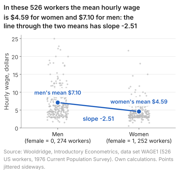
Section 1's first question compares women and men with the same schooling, experience and tenure. By lesson 12's reading, a coefficient in a multiple regression is the difference in predicted \(Y\) between two observations one unit apart in that regressor and equal in every other regressor in the model; for a dummy, the one unit is the step between the groups. The table adds educ (years of schooling), exper (years of potential experience) and tenure (years with the current employer).
| Regressor | Coefficient | Std. error | 95% interval |
|---|---|---|---|
| female (1 = woman) | -1.811 | 0.265 | -2.331 to -1.291 |
| educ | 0.572 | 0.049 | 0.475 to 0.668 |
| exper | 0.025 | 0.012 | 0.003 to 0.048 |
| tenure | 0.141 | 0.021 | 0.099 to 0.183 |
| constant | -1.568 | 0.725 | -2.991 to -0.145 |
Wage in dollars an hour; n = 526 workers; R-squared 0.364.
In these 526 workers a woman's predicted wage is 1.81 dollars an hour below that of a man with the same schooling, experience and tenure (95% interval 1.29 to 2.33 dollars below), against 2.51 dollars with nothing held fixed. Women in this sample average less of all three, above all less tenure (3.62 years against 6.47), and each of the three goes with higher pay in the longer regression. Hence the gap narrows by 0.70 dollars; lesson 13's identity splits the 0.70 among them, 0.40 of it for tenure. Both gaps are comparisons, not measures of what being a woman does to pay: whatever else differs between the two groups and moves pay sits in the error.
R: the code
library(wooldridge)
data("wage1")
fit <- lm(wage ~ female + educ + exper + tenure, data = wage1)
summary(fit)
confint(fit)
R: what it prints
> library(wooldridge)
> data("wage1")
> fit <- lm(wage ~ female + educ + exper + tenure, data = wage1)
> summary(fit)

Call:
lm(formula = wage ~ female + educ + exper + tenure, data = wage1)

Residuals:
    Min      1Q  Median      3Q     Max
-7.7675 -1.8080 -0.4229  1.0467 14.0075

Coefficients:
            Estimate Std. Error t value Pr(>|t|)
(Intercept) -1.56794    0.72455  -2.164   0.0309 *
female      -1.81085    0.26483  -6.838 2.26e-11 ***
educ         0.57150    0.04934  11.584  < 2e-16 ***
exper        0.02540    0.01157   2.195   0.0286 *
tenure       0.14101    0.02116   6.663 6.83e-11 ***
---
Signif. codes:  0 ‘***’ 0.001 ‘**’ 0.01 ‘*’ 0.05 ‘.’ 0.1 ‘ ’ 1

Residual standard error: 2.958 on 521 degrees of freedom
Multiple R-squared:  0.3635,	Adjusted R-squared:  0.3587
F-statistic:  74.4 on 4 and 521 DF,  p-value: < 2.2e-16

> confint(fit)
                   2.5 %      97.5 %
(Intercept) -2.991339439 -0.14453795
female      -2.331108647 -1.29059572
educ         0.474580247  0.66842930
exper        0.002667392  0.04812434
tenure       0.099432346  0.18257778
Python: the code
import wooldridge
import statsmodels.formula.api as smf

wage1 = wooldridge.data("wage1")
fit = smf.ols("wage ~ female + educ + exper + tenure", data=wage1).fit()
print(fit.summary())
Python: what it prints
                            OLS Regression Results
==============================================================================
Dep. Variable:                   wage   R-squared:                       0.364
Model:                            OLS   Adj. R-squared:                  0.359
Method:                 Least Squares   F-statistic:                     74.40
Date:                Sun, 18 Oct 2026   Prob (F-statistic):           7.30e-50
Time:                        00:14:19   Log-Likelihood:                -1314.2
No. Observations:                 526   AIC:                             2638.
Df Residuals:                     521   BIC:                             2660.
Df Model:                           4
Covariance Type:            nonrobust
==============================================================================
                 coef    std err          t      P>|t|      [0.025      0.975]
------------------------------------------------------------------------------
Intercept     -1.5679      0.725     -2.164      0.031      -2.991      -0.145
female        -1.8109      0.265     -6.838      0.000      -2.331      -1.291
educ           0.5715      0.049     11.584      0.000       0.475       0.668
exper          0.0254      0.012      2.195      0.029       0.003       0.048
tenure         0.1410      0.021      6.663      0.000       0.099       0.183
==============================================================================
Omnibus:                      185.864   Durbin-Watson:                   1.794
Prob(Omnibus):                  0.000   Jarque-Bera (JB):              715.580
Skew:                           1.589   Prob(JB):                    4.11e-156
Kurtosis:                       7.749   Cond. No.                         141.
==============================================================================

Notes:
[1] Standard Errors assume that the covariance matrix of the errors is correctly specified.
The code loads WAGE1 from the wooldridge package in R or Python; female is 1 for a woman and 0 for a man.
3. The base group and the intercept
Every dummy coefficient is measured from the base group, so a reading names the base group each time: with female in the model it is men. Which group is coded 1 is a choice that changes the numbers printed, not the comparison. With \(\text{nonsmoker}_i = 1\) if the mother smoked no cigarettes and 0 if she smoked at least one a day, the births give:
| Birthweight regressed on | Base group | Intercept | Coefficient | R-squared |
|---|---|---|---|---|
| smoker (1 = smoked) | non-smokers | 120.061 | -8.915 | 0.0248 |
| nonsmoker (1 = did not smoke) | smokers | 111.146 | 8.915 | 0.0248 |
The intercept is now the smokers' mean, and the coefficient has flipped its sign and kept its size; the fitted values, the residuals and R-squared are unchanged. Section 7 shows that in a log model the swap also changes the size of the exact percentage.
With other regressors, the intercept is the base group's predicted value with every other regressor at zero: in section 2's wage regression, -1.57 dollars an hour for a man with no schooling, experience or tenure. No worker in the sample has all three at zero (the least experienced have one year), and the negative wage shows how far outside the data that point lies. A 0/1 outcome, rather than a regressor, is a different subject (the linear probability model, probit and logit), not covered here.
4. Several categories: four regions, three dummies
In a regression with an intercept, a variable with more than two categories enters as dummies, one fewer than the categories, each compared with the category left out. WAGE1 records which of four US regions each worker lives in: \(\text{northcen}_i = 1\) if worker \(i\) lives in the North Central region and 0 otherwise, and \(\text{south}_i\) and \(\text{west}_i\) likewise; a Northeast worker has all three at 0, so the Northeast is the base group. The outcome is the log wage. Throughout the lesson "log" means the natural logarithm, written \(\ln\), and a difference in log wage is in log points: the mean log wage is 1.678 in the Northeast and 1.609 in North Central, 0.069 log points apart. The regression is
$$ \begin{aligned} \ln(\text{wage}_i) &= \beta_0 + \beta_1\,\text{educ}_i + \beta_2\,\text{exper}_i \\ &\quad + \beta_3\,\text{tenure}_i + \beta_4\,\text{northcen}_i \\ &\quad + \beta_5\,\text{south}_i + \beta_6\,\text{west}_i + u_i . \end{aligned} $$| Region | Workers | Dummy | Coefficient (log points, against the Northeast) | 95% interval |
|---|---|---|---|---|
| Northeast | 118 | none: the base group | 0 | |
| North Central | 132 | northcen | -0.0708 | -0.1804 to 0.0389 |
| South | 187 | south | -0.0477 | -0.1501 to 0.0546 |
| West | 89 | west | 0.0612 | -0.0602 to 0.1827 |
n = 526 workers (118 + 132 + 187 + 89).
In these 526 workers, each coefficient compares a region with the Northeast at the same schooling, experience and tenure: a North Central worker's predicted log wage is 0.071 lower, a Western worker's 0.061 higher, and none of the three intervals excludes zero. Two regions that both have a dummy are compared through the difference of their coefficients: the West against North Central is 0.0612 - (-0.0708) = 0.1320 log points. Its standard error depends on how the two estimates vary together, so it is not in the table; software reports it (0.0604; 95% interval 0.0134 to 0.2506), or the regression can be refitted with one of the two as the base group.
5. The dummy variable trap
A dummy for every category, together with an intercept, leaves least squares without a single answer. Add \(\text{northeast}_i = 1\) for a worker in the Northeast and 0 otherwise. Each worker lives in exactly one region, so for every worker
$$ \begin{aligned} &\text{northeast}_i + \text{northcen}_i \\ &\quad + \text{south}_i + \text{west}_i = 1 , \end{aligned} $$which is the intercept's column. Adding any number \(c\) to all four region coefficients and subtracting \(c\) from the intercept leaves every fitted value unchanged, since each worker has one region dummy equal to 1, and so leaves the sum of squared residuals unchanged. No single set of coefficients minimises the sum: the regressors are perfectly collinear.
R, given all four dummies and an intercept, drops the one listed last: it prints "Coefficients: (1 not defined because of singularities)" and NA (not available) for northeast when it is listed last, or for west when northeast comes first, which makes the West the base group.
| Coefficient | northeast listed last (base: Northeast) | northeast listed first (base: West) |
|---|---|---|
| intercept | 0.30930 | 0.37051 |
| northeast | NA | -0.06121 |
| northcen | -0.07078 | -0.13199 |
| south | -0.04774 | -0.10895 |
| west | 0.06121 | NA |
Five decimals. The two fits have the same coefficients on educ, exper and tenure (0.09182, 0.00427 and 0.02197) and the same fitted values.
The second column is the first shifted by the West's 0.06121: the intercept rises by it, from 0.30930 to 0.37051, and each region's coefficient falls by it, so the gaps between regions are unchanged (North Central against the West is -0.07078 - 0.06121 = -0.13199 in both). Stata's regress also drops one collinear variable and prints a note saying so. The way out is to drop one dummy, whose category becomes the base group, or the intercept, so that each region's coefficient is its own intercept. Two categories fall into the same trap: with \(\text{male}_i = 1\) for a man, \(\text{female}_i + \text{male}_i = 1\) for every worker.
6. A logged outcome: coefficients as percentages
Logging the outcome turns a coefficient from a difference in the units of \(Y\) into an approximate proportional difference in \(Y\). Lesson 11 read the regression of birthweight on cigarettes a day in ounces: in these 1,388 births, 0.514 ounces lower per cigarette. With the log of birthweight as the outcome,
$$ \widehat{\ln(\text{bwght})}_i = 4.7694 - 0.00449\,\text{cigs}_i , $$so one more cigarette a day goes with a predicted log birthweight 0.00449 lower. We want that as a percentage of birthweight. The fitted model is linear on the log scale, so one more cigarette changes the predicted log birthweight by the coefficient, \(b\), wherever it starts, and undoing the log turns that difference into a ratio: if the predicted log birthweight goes from \(\hat y_0\) to \(\hat y_1 = \hat y_0 + b\), then \(e^{\hat y_1} / e^{\hat y_0} = e^{b}\). Hence the exact percentage difference is
$$ 100\,\big(e^{b} - 1\big) . $$In words: exact percentage change in \(Y\) = 100 × (e raised to the coefficient, minus 1).
For \(b\) near zero, \(e^{b}\) is close to \(1 + b\) (the part left out is about \(b^2/2\)), so \(100b\) is close to the exact figure; read the other way, a 5% rise is \(\ln 1.05 = 0.0488\) log points. Here \(100 \times (-0.00449) = -0.449\): about 0.45% lower birthweight per cigarette a day, exactly \(100\,(e^{-0.00449} - 1) = -0.448\%\). For 20 cigarettes a day against none, the predicted log birthweight is \(20 \times 0.00449 = 0.0898\) lower: about 8.98% lower birthweight, exactly \(100\,(e^{-0.0898} - 1) = -8.59\%\), 0.39 percentage points apart. The gap grows with the size of the log difference (the explainer's table of exact against approximate percentages).
The coefficient times 100 is about the percentage change in birthweight per cigarette a day. It is not in ounces: 0.449% of the mean birthweight, 118.70 ounces, is 0.53 ounces, near the 0.514 of the levels regression, a different model. Nor is it in percentage points, the unit for a difference between two rates (per cent against percentage points). With family income held fixed as well, the coefficient is -0.00403: about 0.40% lower birthweight per cigarette for mothers with the same family income, exactly \(100\,(e^{-0.00403} - 1) = -0.402\%\).
When the regressor is logged too, the coefficient is an elasticity, the approximate percentage change in \(Y\) with a 1% change in \(X\), the same at every point. In 209 US firms (1990), a 1% larger firm by sales goes with about 0.26% higher pay for its chief executive. The explainer sets out all four combinations of levels and logs and when to leave a variable in levels. A variable with zeros or negative values has no log, and an error variance that changes with \(X\) is not a reason to take logs, since logging changes the question the regression answers.
7. A dummy in a log model
A dummy in a model for a logged outcome gives a percentage gap between the groups, and at the size of the sex gap in pay the exact figure differs visibly from the rough one. The table gives log wage on female, educ, exper and tenure.
| Regressor | Coefficient | Std. error | 95% interval |
|---|---|---|---|
| female (1 = woman) | -0.3011 | 0.0372 | -0.3743 to -0.2280 |
| educ | 0.0875 | 0.0069 | 0.0738 to 0.1011 |
| exper | 0.0046 | 0.0016 | 0.0014 to 0.0078 |
| tenure | 0.0174 | 0.0030 | 0.0115 to 0.0232 |
| constant | 0.5013 | 0.1019 | 0.3012 to 0.7015 |
Log wage; n = 526 workers; R-squared 0.392.
In these 526 workers, the female coefficient of log wage on female, educ, exper and tenure, -0.3011, puts a woman's predicted log wage 0.301 below that of a man with the same schooling, experience and tenure: about 30.1% lower pay by the rough reading. The exact reading uses the ratio of the two predicted wages, \(e^{b}\), which is 0.7400 with \(b\) carried to five decimals (the second row of the table below). So a woman's predicted wage is 26.00% below a comparable man's, and the rough reading is 4.1 percentage points further from zero. The coefficient's 95% interval converts the same way, to a gap of 20.39% to 31.22%.
With \(\text{male}_i = 1\) for a man and 0 for a woman in place of female, the coefficient keeps its size and changes sign, as in section 3, but the exact figure changes more than its sign. Now \(e^{b}\) is 1.3514, so a man's predicted wage is 35.14% above a comparable woman's. The ratios are reciprocals, \(1/0.7400 = 1.3514\): the base group is the denominator of the percentage, a second reason to name it with every reading.
| Model for log wage | Dummy (base group) | b | About 100b | Exactly 100(eb - 1) |
|---|---|---|---|---|
| on educ and female | female (men) | -0.36087 | -36.1% | -30.29% |
| on female, educ, exper, tenure | female (men) | -0.30115 | -30.1% | -26.00% |
| on male, educ, exper, tenure | male (women) | 0.30115 | 30.1% | 35.14% |
Coefficients to five decimals, so that each row's arithmetic reproduces.
The first row holds only schooling fixed, and its gap is wider for the reason section 2 gave in dollars. Section 4's North Central coefficient, -0.07078 to five decimals, reads the same way: about 7.1% lower pay than in the Northeast, exactly 6.83%. For a coefficient of 0.05 the readings are 5.00% and 5.13%; the explainer's table shows the gap growing with the coefficient.
8. Interactions: a slope that depends on another regressor
An interaction lets the slope on one regressor depend on the value of another, through their product entered as a regressor with its own coefficient. So far schooling has had one coefficient for both sexes, so the women's predicted log wage lay below the men's by the same amount at every level of schooling: an assumption of the model, as lesson 12 noted, not a finding.
Definition: interaction term
An interaction term is the product of two regressors, \(X_{1i} X_{2i}\), entered with a coefficient of its own:
$$ \begin{aligned} Y_i &= \beta_0 + \beta_1 X_{1i} + \beta_2 X_{2i} \\ &\quad + \beta_3 X_{1i} X_{2i} + u_i . \end{aligned} $$Compare \(X_1 = x_1\) with \(X_1 = x_1 + 1\), with \(X_2 = x_2\) in both. The terms \(\beta_0\) and \(\beta_2 x_2\) do not change, \(\beta_1 x_1\) rises by \(\beta_1\), and \(\beta_3 x_1 x_2\) rises by \(\beta_3 x_2\). So the slope of \(Y\) on \(X_1\) is
$$ \beta_1 + \beta_3 X_2 . $$In words: slope on \(X_1\) = coefficient on \(X_1\) + interaction coefficient × the value of \(X_2\).
Remarks. \(\beta_1\) on its own is the slope of \(Y\) on \(X_1\) where \(X_2 = 0\), and \(\beta_2\) on its own is the difference in \(Y\) per unit of \(X_2\) where \(X_1 = 0\). Neither is an average over the data, and a value of 0 may lie outside the data. Books call \(\beta_1\) and \(\beta_2\) "main effects", a name that hides both points. When \(X_2\) is a dummy, \(X_2 = 0\) is the base group: with \(X_2 = \text{female}\), \(\beta_1\) is the men's slope and \(\beta_1 + \beta_3\) the women's.
For the wages, educ_female = educ × female is a woman's years of schooling and 0 for a man. The table gives log wage on educ, female, educ_female, exper and tenure.
| Regressor | Coefficient | Std. error | 95% interval |
|---|---|---|---|
| educ | 0.0903 | 0.0087 | 0.0732 to 0.1074 |
| female (1 = woman) | -0.2104 | 0.1740 | -0.5521 to 0.1314 |
| educ_female | -0.0072 | 0.0136 | -0.0339 to 0.0194 |
| exper | 0.0046 | 0.0016 | 0.0014 to 0.0078 |
| tenure | 0.0174 | 0.0030 | 0.0116 to 0.0233 |
| constant | 0.4647 | 0.1229 | 0.2233 to 0.7061 |
Log wage; n = 526 workers; R-squared 0.393.
The coefficient on educ, 0.0903, is the men's slope (female = 0): in these 526 workers, among men alike in experience and tenure, a year more schooling goes with about 9.0% higher predicted pay. The women's slope adds the coefficient on educ_female: 0.090276 + (-0.007245) = 0.083031, or 0.0830 to four decimals, about 8.3% a year. (The working carries six decimals because the table's rounded 0.0903 and -0.0072 add to 0.0831.)
The coefficient on female, -0.2104, is no longer the sex gap but, by the definition, the gap where educ = 0, at the same experience and tenure. Only 2 of the 526 workers have no schooling, both women, and 18 have fewer than 8 years. At 12 years, which 198 workers report, more than any other figure, the gap is -0.2104 + 12 × (-0.0072) = -0.297 log points (standard error 0.038).
R: the code
library(wooldridge)
data("wage1")
wage1$educ_female <- wage1$educ * wage1$female
fit <- lm(lwage ~ educ + female + educ_female + exper + tenure, data = wage1)
summary(fit)
confint(fit)
R: what it prints
> library(wooldridge)
> data("wage1")
> wage1$educ_female <- wage1$educ * wage1$female
> fit <- lm(lwage ~ educ + female + educ_female + exper + tenure, data = wage1)
> summary(fit)

Call:
lm(formula = lwage ~ educ + female + educ_female + exper + tenure,
    data = wage1)

Residuals:
     Min       1Q   Median       3Q      Max
-1.91695 -0.26530 -0.02059  0.25715  1.27586

Coefficients:
             Estimate Std. Error t value Pr(>|t|)
(Intercept)  0.464712   0.122892   3.781 0.000174 ***
educ         0.090276   0.008715  10.359  < 2e-16 ***
female      -0.210376   0.173969  -1.209 0.227107
educ_female -0.007245   0.013562  -0.534 0.593456
exper        0.004642   0.001628   2.850 0.004541 **
tenure       0.017436   0.002981   5.849 8.76e-09 ***
---
Signif. codes:  0 ‘***’ 0.001 ‘**’ 0.01 ‘*’ 0.05 ‘.’ 0.1 ‘ ’ 1

Residual standard error: 0.4162 on 520 degrees of freedom
Multiple R-squared:  0.3926,	Adjusted R-squared:  0.3868
F-statistic: 67.22 on 5 and 520 DF,  p-value: < 2.2e-16

> confint(fit)
                   2.5 %      97.5 %
(Intercept)  0.223285941 0.706137381
educ         0.073154475 0.107396796
female      -0.552143591 0.131392139
educ_female -0.033888561 0.019399387
exper        0.001442415 0.007840616
tenure       0.011579418 0.023292197
Python: the code
import wooldridge
import statsmodels.formula.api as smf

wage1 = wooldridge.data("wage1")
wage1["educ_female"] = wage1["educ"] * wage1["female"]
fit = smf.ols("lwage ~ educ + female + educ_female + exper + tenure", data=wage1).fit()
print(fit.summary())
Python: what it prints
                            OLS Regression Results
==============================================================================
Dep. Variable:                  lwage   R-squared:                       0.393
Model:                            OLS   Adj. R-squared:                  0.387
Method:                 Least Squares   F-statistic:                     67.22
Date:                Sun, 18 Oct 2026   Prob (F-statistic):           3.98e-54
Time:                        00:14:20   Log-Likelihood:                -282.31
No. Observations:                 526   AIC:                             576.6
Df Residuals:                     520   BIC:                             602.2
Df Model:                           5
Covariance Type:            nonrobust
===============================================================================
                  coef    std err          t      P>|t|      [0.025      0.975]
-------------------------------------------------------------------------------
Intercept       0.4647      0.123      3.781      0.000       0.223       0.706
educ            0.0903      0.009     10.359      0.000       0.073       0.107
female         -0.2104      0.174     -1.209      0.227      -0.552       0.131
educ_female    -0.0072      0.014     -0.534      0.593      -0.034       0.019
exper           0.0046      0.002      2.850      0.005       0.001       0.008
tenure          0.0174      0.003      5.849      0.000       0.012       0.023
==============================================================================
Omnibus:                       12.292   Durbin-Watson:                   1.774
Prob(Omnibus):                  0.002   Jarque-Bera (JB):               23.057
Skew:                           0.015   Prob(JB):                     9.85e-06
Kurtosis:                       4.025   Cond. No.                         271.
==============================================================================

Notes:
[1] Standard Errors assume that the covariance matrix of the errors is correctly specified.
The code makes the product, educ_female = educ × female, before fitting the regression.
9. A dummy times a continuous regressor: two lines
A dummy times a continuous regressor gives two fitted lines, each with its own intercept and slope. At zero experience and tenure the men's line is 0.4647 + 0.0903 educ, and the women's has intercept 0.4647 - 0.2104 = 0.2543 and slope 0.0830. Figure 2 draws the lines with experience and tenure at their sample means, 17.0 and 5.1 years, where the intercepts are 0.633 and 0.422; the slopes do not depend on where experience and tenure are held.
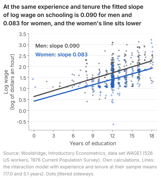
The women's fitted line is flatter, but the interaction coefficient's 95% interval, -0.0339 to 0.0194 (standard error 0.0136, p = 0.593), contains zero: these 526 workers give no evidence that the slope of log wage on schooling differs between men and women. Nor does the interval show the slopes equal, since it also contains a women's slope 0.033 below the men's.
With the slopes as estimated, the gap widens with schooling: a woman's predicted log wage is 0.268 below a comparable man's at 8 years, 0.297 at 12 and 0.326 at 16 (standard errors 0.072, 0.038 and 0.060). At 12 years it is close to the -0.3011 of section 7's model (log wage on female, educ, exper and tenure), whose lines are parallel. So the model separates two claims: that the women's line is lower (at 8, 12 and 16 years of schooling the gap is more than three standard errors from zero) and that it is flatter (a difference in slopes, for which these data give no evidence). Separate regressions for the 274 men and the 252 women give slopes of 0.0963 and 0.0800 instead, because they also give experience and tenure their own coefficients for each sex; the two routes agree only when every regressor is interacted with female.
10. Common mistakes
- "The coefficient on female is what being a woman does to pay." It compares women and men alike in the regressors: 1.81 dollars an hour lower at the same schooling, experience and tenure. Whatever else differs between them and moves pay is in the error.
- "A dummy's coefficient is the mean of the group coded 1." With no other regressor, it is that group's mean minus the base group's: -2.51 is 4.59 - 7.10.
- "Four categories need four dummies." With an intercept, four region dummies add up to its column of ones and least squares has no unique solution; R prints NA for one. Use three, and name the base group.
- "A log coefficient of -0.00449 means 0.00449% lower." Multiply by 100: about 0.45% lower birthweight per cigarette a day.
- "If women earn 26.00% less than men, men earn 26.00% more than women." The two ratios are reciprocals, 0.7400 one way and 1/0.7400 = 1.3514 the other: a man's predicted wage is 35.14% above a comparable woman's.
- "With an interaction in the model, the female coefficient is the sex gap." It is the gap at zero years of schooling, -0.2104; at 12 years the gap is -0.297.
- "The interaction is not significant, so the two slopes are equal." Its interval, -0.0339 to 0.0194, contains zero and also a women's slope 0.033 below the men's.
11. Check your understanding
Five questions, marked on the page; every option has an explanation, including the wrong ones. (Without JavaScript the explanations are shown beneath each question.)
1. For 526 US workers (1976), log wage is regressed on educ, exper, tenure and three region dummies, with the Northeast as the base group. The coefficient on south (1 for a worker in the South, 0 otherwise) is -0.0477. For workers with the same schooling, experience and tenure, which reading is right?
A dummy's coefficient compares its group with the base group: here the Northeast's 118 workers, who have all three region dummies at 0. The mean of all 526 workers, the South's 187 included, plays no part in it.
-0.048 is not the South's level of log wage: its 187 workers have a mean log wage of 1.559. A dummy's coefficient is the difference between its group's predicted value and the base group's, not the group's own value.
Correct. The Northeast is the base group, so each region's coefficient compares that region with it, at the same schooling, experience and tenure: -0.0477 log points is about 4.8% lower pay. Its 95% interval, -0.1501 to 0.0546, contains zero, so the data are also compatible with no difference.
2. Among the 526 workers, mean tenure (years with the current employer) is 6.474 for the 274 men and 3.615 for the 252 women. Tenure is regressed on an intercept and female (1 for a woman, 0 for a man). What is the estimated intercept?
3.615 - 6.474 = -2.859 is the women's mean minus the men's. That is the coefficient on female, not the intercept.
3.615 is the mean of the group coded 1, the women. Their predicted tenure is the intercept plus the coefficient: 6.474 + (-2.859) = 3.615.
5.105 years is the mean tenure of all 526 workers. With a dummy in the model, the intercept is not the overall mean but the mean of the base group.
Correct. In a regression on one dummy, least squares puts the fitted value of each group at that group's mean. The base group is men (female = 0), so the intercept is their mean, 6.474 years, and the coefficient on female is 3.615 - 6.474 = -2.859.
3. Each of the 526 workers lives in one of four US regions: Northeast, North Central, South or West. A regression of log wage on an intercept, educ, exper and tenure is to compare the four regions. Which region regressors does it need?
Correct. With an intercept in the model, a variable with four categories needs three dummies. Each coefficient compares its region with the one left out, so the lesson's choice, northcen, south and west, makes the Northeast's 118 workers the base group.
The four dummies add up to 1 for every worker, which is the intercept's column, so least squares has no unique solution: R prints NA for one of them. Leaving one region out loses nothing, since its workers are the base group that the other three are compared with.
A single code forces the predicted log wage to change by the same amount from region 1 to 2, from 2 to 3 and from 3 to 4, an order and a spacing the regions do not have. Three dummies let each region differ from the base group by its own amount.
4. A student regresses wage on an intercept, female (1 for a woman, 0 for a man) and male (1 for a man, 0 for a woman), using the 526 workers. What goes wrong?
That reading needs a constraint on the coefficients that ordinary least squares does not impose. With an intercept, female and male, the fit has no unique solution, and R prints NA for one of the three.
-2.51 and +2.51 are the gap seen from each side, which two separate regressions would give, one on female and one on male. In one regression with an intercept the two dummies add up to 1 for every worker, so no unique set of coefficients exists.
Correct. Every worker is either a woman or a man, so female + male = 1 for all 526, which is the intercept's column. Adding any number to both dummy coefficients and subtracting it from the intercept leaves every fitted value unchanged, so least squares has no unique solution. Drop one dummy, or the intercept.
5. In the regression of log wage on educ, exper, tenure and three region dummies (the Northeast the base group), the coefficient on west (1 for a worker in the West, 0 otherwise) is 0.0612. How does a Western worker's predicted pay compare with that of a Northeastern worker with the same schooling, experience and tenure?
The outcome is the log wage, so the coefficient is a difference in log points, not in dollars. A difference of 0.0612 in log wage is a percentage difference in pay: about 6.1%.
Correct. In a log model a coefficient b on a dummy is a difference of b in predicted log wage, which is about 100b per cent: 100 × 0.0612 = 6.1%. Exactly, it is \(100\,(e^{0.0612} - 1)\) = 6.31%. Its 95% interval, -0.0602 to 0.1827, contains zero, so the data are also compatible with no difference.
Percentage points measure the difference between two rates or shares, and pay is not a rate. 0.0612 log points is a percentage difference in pay, about 6.1%, not a difference of 6.1 points in anything.
12. Three questions about dummies, logs and interactions
A dummy variable coefficient is the difference in the predicted outcome between the group coded 1 and the base group, coded 0, with the other regressors held fixed. In 526 US workers (1976), the coefficient on female is -1.81: a woman's predicted wage is 1.81 dollars an hour below that of a man with the same schooling, experience and tenure.
The dummy variable trap is putting a dummy for every category into a regression that also has an intercept. The dummies add up to the intercept's column of ones, so least squares has no unique solution, and R reports NA for one of them. With four regions, use three dummies; the fourth region becomes the base group.
An interaction coefficient is how much the slope on one regressor changes per unit of the other. With log wage on schooling, female, their product, experience and tenure, the schooling slope is 0.090 for men and 0.090 - 0.007 = 0.083 for women. The female coefficient alone is then the gap at zero schooling, not an average gap.
13. Where next
- Logs and elasticities in regression, the explainer: all four combinations of levels and logs, the exact against approximate table, elasticities, and when not to take logs.
- Lesson 15 on the course home: heteroskedasticity and robust standard errors, the next lesson of Part 4.
- How to read regression output, for every column of a printout such as those of sections 2 and 8.
- Lesson 13: omitted variable bias, for the identity that accounts for the move of the female coefficient from -2.51 to -1.81 when schooling, experience and tenure were added.
Stuck on a dummy, log or interaction coefficient? Send it
I tutor statistics and econometrics one-to-one, from a first regression through to dummies, logs, panel data and time series. Bring the printout or the question you are stuck on and we will work through it in the free 30-minute consultation.
Book a free 30-minute consultation Econometrics tutor: how it works
Data. Wages: Wooldridge, Introductory Econometrics: A Modern Approach, data set WAGE1 (526 US workers, 1976 Current Population Survey); results quoted, data not republished. Birthweights: Wooldridge, Introductory Econometrics: A Modern Approach, data set BWGHT (1,388 births, 1988 National Health Interview Survey); a smoker is a mother who smoked at least one cigarette a day during pregnancy; results quoted, data not republished. Chief executive pay (section 6, one number): Wooldridge, Introductory Econometrics: A Modern Approach, data set CEOSAL1 (209 US firms, 1990, a random sample of the data reported in Businessweek of 6 May 1991); results quoted, data not republished. Questions: the same WAGE1 data, with the regressions of this page, the group means of tenure, and one regression in which educ, exper and tenure are each interacted with female. Adapted in part from my lecture notes for Cross-Section Econometrics (ECON60052, 2019) at the University of Manchester.