The four reference distributions of econometric inference are one family built from the normal. Square and sum k independent standard normals and you get a chi-square with k degrees of freedom; divide a normal by the root of a scaled independent chi-square and you get a t; take a ratio of two scaled chi-squares and you get an F. Single coefficient tests use the normal or t; joint restriction tests use the chi-square (large sample) or F (finite sample).
How to read these notes
These notes are for a student who has met hypothesis testing and confidence intervals and keeps meeting these four distributions without seeing how they relate. We start from the normal and build the others from it, then map each distribution to the test that uses it. The relationships, not the density formulas, are what matter.
1. The normal distribution: the foundation
The normal (Gaussian) distribution is the starting point because of the central limit theorem: sample averages, and therefore most estimators, are approximately normally distributed in large samples regardless of the underlying data. A standard normal \(Z \sim N(0,1)\) has mean 0 and variance 1, and its familiar bell shape is the reference for any single standardised estimate.
This is why \(\pm 1.96\) appears everywhere: 95% of the standard normal distribution lies within 1.96 of zero. Every other distribution in this note is constructed by manipulating independent standard normals.
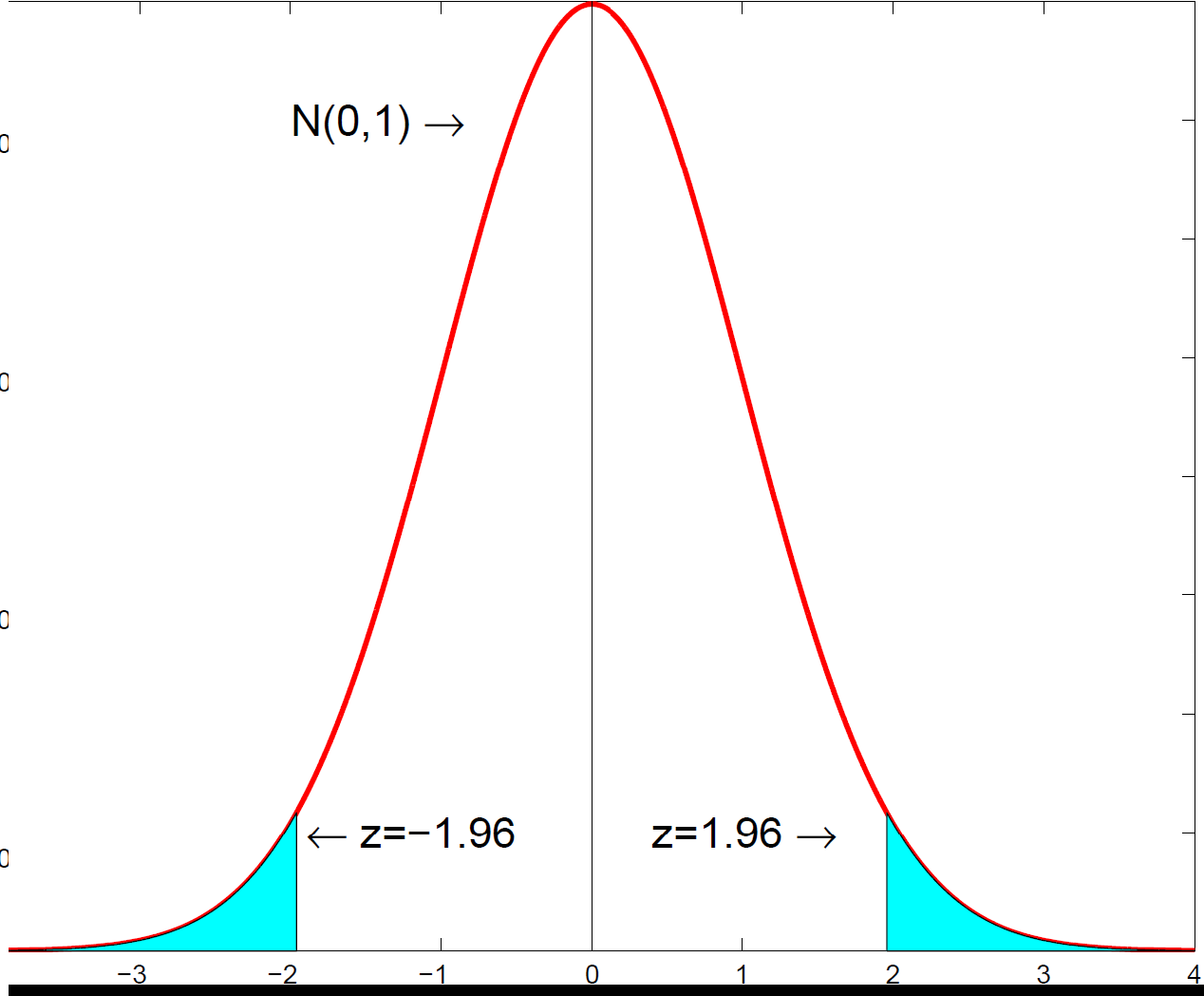 The standard normal density, the building block from which the t, chi-square and F distributions are all constructed.
2. The chi-square distribution: squaring and summing
The chi-square distribution arises whenever we add up squared normals. The definition is exactly that.
For \(k\) independent standard normal variables \(X_1, \dots, X_k \sim N(0,1)\), the sum of their squares has a chi-square distribution with \(k\) degrees of freedom: \(\sum_{j=1}^{k} X_j^2 \sim \chi^2_k\).
Because it is a sum of squares, a chi-square variable is always non-negative and its distribution is right-skewed, with the skew shrinking as the degrees of freedom \(k\) grow. The plot below shows \(\chi^2_k\) for \(k = 1, 5, 10\): more degrees of freedom shift the mass to the right and make the shape more symmetric.
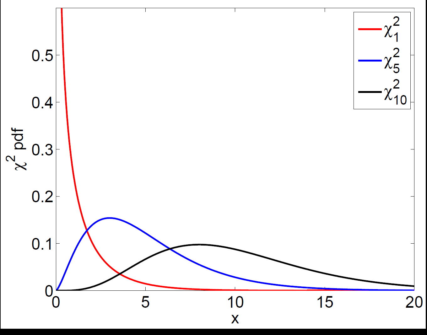 Chi-square densities for k = 1, 5, 10 degrees of freedom; the distribution is non-negative and becomes more symmetric as k increases.
The chi-square is the natural distribution for testing several things at once, because a joint test typically squares and adds up several standardised quantities. For example, the Q-test for whether a set of autocorrelations are jointly zero sums squared sample autocorrelations and is compared against a \(\chi^2\).
3. The t-distribution: a normal over a chi-square
The Student t-distribution appears when we standardise a normal estimate but have to estimate the variance rather than knowing it. Formally, a t-variable is a standard normal divided by the square root of an independent chi-square scaled by its degrees of freedom:
Estimating the error variance adds uncertainty, which fattens the tails relative to the normal. The t-distribution captures that. With few degrees of freedom its tails are noticeably heavier; as \(k \to \infty\) the estimated variance settles down and the t-distribution converges to the standard normal.
This is the distribution behind the t-statistic used to test a single regression coefficient. In large samples the difference from the normal is negligible — which is why the 1.96 rule still works — but in small samples the exact t critical value is larger.
4. The F-distribution: a ratio of two chi-squares
The F-distribution is the ratio of two independent chi-squares, each divided by its own degrees of freedom:
It has two degrees-of-freedom parameters — one for the numerator (\(m\)) and one for the denominator (\(n\)) — and like the chi-square it is non-negative and right-skewed. The F-distribution is what you use to test a joint hypothesis about several coefficients in finite samples, such as "these \(p\) variables are all zero". The numerator measures the improvement in fit from relaxing the restrictions; the denominator is the unexplained variance.
The chi-square and F tests of joint restrictions are two versions of the same idea. The chi-square form is the large-sample (asymptotic) version; the F form is the finite-sample version used when the errors are normal. In large samples \(m \times F_{m,n} \approx \chi^2_m\), so they agree. Packages typically report the F-test for joint coefficient restrictions.
5. How they all connect
The four distributions are not separate facts to memorise — they are one chain of constructions starting from the normal.
- Square a standard normal and you get \(\chi^2_1\). Sum \(k\) of them and you get \(\chi^2_k\).
- Divide a standard normal by the root of a scaled independent chi-square and you get a t.
- Take a ratio of two scaled chi-squares and you get an F.
- A useful special case ties the last two together: \(t_k^2 = F_{1,k}\). Squaring a t-statistic gives an F with one numerator degree of freedom, which is why a two-sided t-test and the corresponding single-restriction F-test always give the same answer.
6. Which distribution does which test use?
The practical pay-off is knowing, when you see a test statistic, which table (or which p-value) it should be compared against.
| Test | What it checks | Reference distribution |
|---|---|---|
| z-test | A single coefficient or mean, variance known / large sample | Standard normal \(N(0,1)\) |
| t-test | A single coefficient, variance estimated | Student \(t_k\) |
| F-test | Several coefficient restrictions jointly (finite sample) | \(F_{m,n}\) |
| Chi-square / LR / LM / Q-test | Several restrictions jointly (large sample) | \(\chi^2_k\) |
So the rule of thumb is: one restriction → normal or t; many restrictions → chi-square or F. The chi-square versions (the likelihood-ratio and Lagrange-multiplier tests) are the large-sample tools you meet in maximum likelihood and time-series diagnostics, while the t and F are the finite-sample workhorses of ordinary regression.
Statistics & econometrics tuition
The relationships between the normal, t, chi-square and F distributions unlock most of statistical inference once they click. For 1-1 help with distribution theory, test statistics or inference, see statistics tuition, econometrics tuition or university economics tuition.
Free videos: the @economaths channel has worked videos on t-tests, F-tests for linear restrictions and p-values.