A confidence interval is a range of plausible values for a parameter, built as the estimate plus or minus a critical value times the standard error. A t-statistic measures how many standard errors the estimate lies from a hypothesised value. A two-sided t-test rejects exactly the values that fall outside the confidence interval, so the two are the same idea: the interval is the set of null values a test would not reject.
How to read these notes
These notes are for a student who has met OLS and the basics of hypothesis testing and wants to be confident interpreting the standard errors, t-statistics and intervals that regression output reports. We work with a single coefficient throughout, but the logic carries over to any estimate with a known standard error.
1. An estimate needs a measure of uncertainty
Suppose we estimate a regression coefficient and obtain \(\hat\beta = 0.42\). On its own this number tells us little, because a different sample would have produced a different estimate. The estimate \(\hat\beta\) is a draw from a sampling distribution centred (under the right assumptions) on the true value \(\beta\). To say anything useful we need to quantify how spread out that sampling distribution is. That measure is the standard error.
The standard error \(\operatorname{se}(\hat\beta)\) is the estimated standard deviation of the sampling distribution of \(\hat\beta\). A small standard error means the estimate would change little from sample to sample, so it is precise; a large standard error means it is imprecise.
The key theoretical fact, delivered by the central limit theorem, is that in large samples the standardised estimate is approximately standard normal:
Everything that follows — both confidence intervals and t-tests — is built on this single result.
2. Building a confidence interval
Because the standardised estimate is approximately \(N(0,1)\), and a standard normal variable lies between \(-1.96\) and \(+1.96\) with probability 0.95, we have
Rearranging the inequality to isolate \(\beta\) turns this into a statement about an interval around the estimate. The 95% confidence interval is
The number 1.96 is the critical value; for a 90% interval it would be 1.645, and for a 99% interval 2.576. A wider confidence level needs a wider interval. So if \(\hat\beta = 0.42\) with a standard error of 0.10, the 95% interval runs from roughly 0.22 to 0.62.
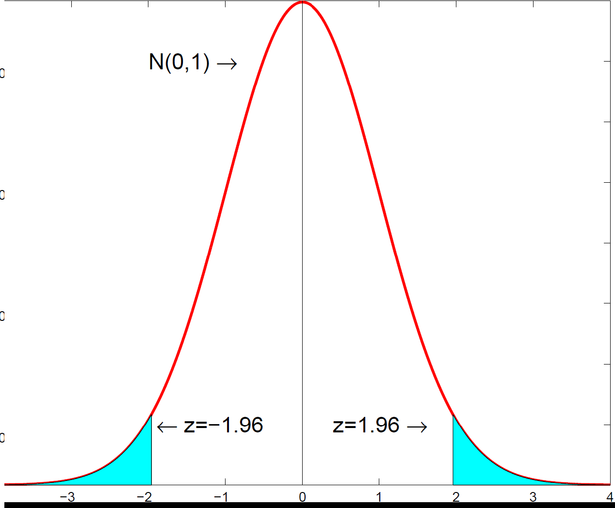 The central 95% of the standard normal distribution lies between the critical values; this is what the confidence interval and the rejection region are built from.
3. What "95% confident" really means
This is the single most misunderstood idea in introductory statistics. The 95% does not mean there is a 95% probability that the true \(\beta\) lies in this particular interval. The true \(\beta\) is a fixed (if unknown) number; once the interval is computed, \(\beta\) is either in it or not.
The 95% refers to the procedure. If we drew many samples and built an interval from each one the same way, about 95% of those intervals would contain the true \(\beta\). Confidence is a property of the method's long-run success rate, not of any single interval.
A useful informal reading is still fair: the interval gives a range of values for \(\beta\) that are plausible given the data. Values inside the interval are consistent with what we observed; values far outside are not.
4. The t-statistic and the t-test
A t-test approaches the same uncertainty from the testing side. To test whether \(\beta\) equals some hypothesised value \(\beta_0\), we form the t-statistic: how many standard errors the estimate lies away from \(\beta_0\).
By far the most common case is testing whether a coefficient is zero — that is, whether the variable matters at all. Setting \(\beta_0 = 0\) gives the t-statistic that regression packages report automatically:
If \(|t| > 1.96\) we reject the null at the 5% level — the estimate is more than about two standard errors from the hypothesised value, which would be unlikely if the null were true. This is why a coefficient roughly twice its standard error is described as "significant".
The p-value reported alongside the t-statistic is the probability of seeing a t-statistic at least this extreme if the null were true; a p-value below 0.05 corresponds to \(|t|>1.96\).
5. Why the "t" and not the "z"
We motivated everything with the standard normal, yet the statistic is called a t-statistic. The reason is that the standard error is itself estimated from the data, which introduces a little extra uncertainty. When the errors are normal, accounting for this exactly gives the Student's t-distribution rather than the normal.
The t-distribution is slightly heavier-tailed than the normal, so its critical values are a bit larger in small samples. With many degrees of freedom it is indistinguishable from the standard normal, which is why the 1.96 rule works well in large samples. In small samples you should use the exact t critical value.
6. The duality: intervals and tests are the same thing
Confidence intervals and two-sided t-tests are not two separate tools — they are the same calculation. Compare them: the test rejects \(\beta_0\) when \(|\hat\beta - \beta_0| > 1.96\,\operatorname{se}(\hat\beta)\), and the confidence interval is exactly the set of values within \(1.96\,\operatorname{se}(\hat\beta)\) of \(\hat\beta\). Therefore:
A two-sided test at the 5% level rejects \(\beta_0\) if and only if \(\beta_0\) lies outside the 95% confidence interval. Equivalently, the confidence interval is the collection of all null values that a two-sided test would not reject at that level.
This has a practical payoff. To check whether a coefficient is significantly different from zero, you can just look at whether zero is inside its confidence interval — if it is not, the coefficient is significant at the corresponding level. The interval also tells you something a bare "reject / do not reject" verdict does not: the range of effect sizes the data are compatible with, which is usually more informative than significance alone.
Statistics & econometrics tuition
Confidence intervals and t-tests are the workhorses of applied statistics, and the place students most often go wrong on interpretation. For 1-1 help with inference, standard errors or reading regression output, see statistics tuition, econometrics tuition or university economics tuition.
Free videos: the @economaths channel has worked videos on regression t-tests, confidence intervals and p-values.